How to Use the FIXED Text Function in Google Sheets

The FIXED function in Google Sheets is specifically designed for formatting numbers with a fixed number of decimal places and optional thousand separators. Since it’s a text function, the formatted numbers are converted into text. This function is particularly useful in reports for consistently displaying financial or numeric data.

When formatting numbers using a formula, you can choose between the TEXT function and the FIXED function. The TEXT function requires a specific format pattern, while the FIXED function applies formatting without needing additional specifications.

Syntax of the FIXED Function in Google Sheets

FIXED(number, [number_of_places], [suppress_separator])

Arguments:

number – The number to be formatted.
number_of_places (optional) – Specifies the number of decimal places to display. The default is 2. If the number has more significant digits than the specified number_of_places, it will be rounded rather than truncated.
suppress_separator (optional) – Determines whether to include the thousand separator. By default, separators are included. Use 1 to exclude them and 0 to keep them.

Formula Examples for the FIXED Function in Google Sheets

1. Using FIXED Without Optional Arguments

The following formula in D2, copied down to D8, converts numbers into text while maintaining thousand separators and rounding to two decimal places:

=FIXED(B2)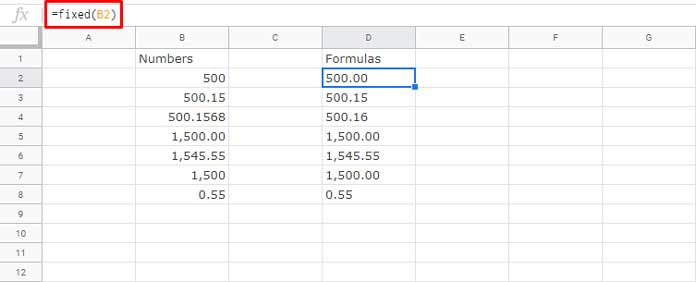

FIXED Function with Two Decimal Places and a Thousand Separator in Google Sheets

This produces the same result as:

=FIXED(B2, 2, 0)

2. Formatting Numbers as Text Without Thousand Separators

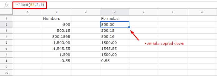
If you want to remove the thousand separator, use the following formula:

=FIXED(B2, 2, 1)

This ensures that numbers are converted to text without commas.

FIXED Function with Two Decimal Places and No Thousand Separator in Google Sheets

Additional Tips for Using the FIXED Function in Google Sheets

Convert FIXED to an Array Formula

The FIXED function is a non-array function, meaning it typically works on individual cells. However, you can convert it into an array formula:

=ArrayFormula(FIXED(B2:B8, 2, 1))

This formula applies the FIXED function across the entire range B2:B8, returning results in D2:D8. If you encounter an error, ensure there are no existing values in D3:D8, as array formulas cannot overwrite existing data.

Using FIXED Formatted Text in Calculations

Since the FIXED function returns text values, you may need a workaround to use the formatted numbers in calculations. Multiply by 1 to convert the text back into numbers:

=SUM(ArrayFormula(FIXED(B2:B8, 2, 1) * 1))

Using the TEXT Function Instead of FIXED

In some cases, the TEXT function may be a better alternative, as it supports multiple formatting patterns. Here’s how to replace FIXED with TEXT:

Example 1: Formatting a Number with Two Decimal Places

=TEXT(1500, "0.00")

Example 2: Formatting with a Thousand Separator

=TEXT(1500, "#,###.00")

This formula handles empty cells differently compared to FIXED. While FIXED returns "0.00", TEXT returns ".00".