")
")


")


")

")
")
 in Excel & Google Sheets")


To find the last occurrence of multiple criteria in Google Sheets, use the FILTER function combined with CHOOSEROWS. This method dynamically retrieves the most recent match without manual sorting.
Where Is This Useful?
If you receive “Apple” multiple times from different vendors, and the same vendors send the item more than once, you might want to find when a vendor last sent “Apple.”
So, the criteria will be the vendor name and item name. Whether the data is sorted or unsorted, the formula should work.
Generic Formula
=CHOOSEROWS(FILTER(data, criteria_column1=condition1, criteria_column2=condition2, [...]), -1)Where:
data– The data range to search in.criteria_column1– First column to apply the condition.criteria_column2– Second column to apply the condition.condition1– The first condition applied incriteria_column1.condition2– The second condition applied incriteria_column2.
You can specify additional criteria columns and conditions.
Handling Unsorted Data
If your data includes a date column and is not sorted by date, modify the formula to include sorting:
=CHOOSEROWS(SORT(FILTER(data, criteria_column1=condition1, criteria_column2=condition2, [...]), sort_column, TRUE), -1)Replace sort_column with the column number of the date column.
Example: Finding the Last Occurrence of Multiple Criteria
Sample Data (A1:D):
| Date | Item | Vendor | Qty |
| 10/01/2024 | Apple | A | 50 |
| 12/02/2024 | Banana | B | 30 |
| 05/03/2024 | Apple | A | 60 |
| 15/04/2024 | Orange | C | 40 |
| 20/05/2024 | Apple | B | 20 |
| 25/06/2024 | Apple | A | 70 |
Formula to Find the Last Receipt of Apple from Vendor A:
=CHOOSEROWS(FILTER(A2:D, B2:B=F2, C2:C=G2), -1)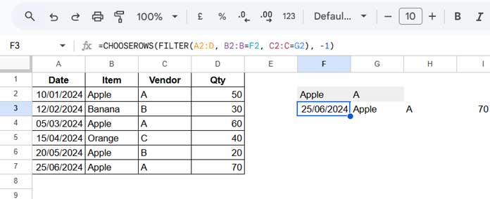
Formula Explanation:
- Filter the Data:
FILTER(A2:D, B2:B=F2, C2:C=G2)– extracts rows whereB2:B = AppleandC2:C = A. - Sort by Date (if needed):
SORT(..., 1, TRUE)– sorts results by date in ascending order. - Get the Last Row:
CHOOSEROWS(..., -1)– extracts the last matching record.
If sorting is necessary:
=CHOOSEROWS(SORT(FILTER(A2:D, B2:B=F2, C2:C=G2), 1, TRUE), -1)FAQ
How Do I Find the Quantity of the Last Occurrence?
Wrap the formula with CHOOSECOLS to return only the quantity column:
=CHOOSECOLS(CHOOSEROWS(SORT(FILTER(A2:D, B2:B=F2, C2:C=G2), 1, TRUE), -1), 4)How Do I Find the First Occurrence Instead?
Replace -1 with 1 in CHOOSEROWS:
=CHOOSEROWS(FILTER(A2:D, B2:B=F2, C2:C=G2), 1)How Do I Find the Last Two Occurrences?
Replace -1 with {-1, -2}:
=CHOOSEROWS(FILTER(A2:D, B2:B=F2, C2:C=G2), {-1, -2})
Superb, Thank you so much. Literally, I have been trying this for quite a long time. Thank you so much for always being very helpful. Looking forward to the explanation.
Hi, Zyshan,
Here is the link.
How to Get LOOKUP Result from a Dynamic Column in Google sheets.
Hello Prashanth,
I am unable to apply the formula to get the last value against the two criteria.
I am sharing a sheet with you so you could easily understand the issue.
I am trying to apply the formula to get the last value from the closing stock by adding two criteria’s cells i.e “date” & ” Raw material name”.
Since I got the desired result but unable to drag that formula to get more results according to the criteria.
Kindly see if you could help me with that.
Sample Sheet – removed by admin –
Hi, Zyshan,
The scenario was not the same as per my tutorial. There are several columns involved. So I have written another formula for you.
You can use this formula in cell E10, then copy-paste down.
=ifna(lookup($D$1,filter({'RM INVENTORY'!$D$8:$D,filter('RM INVENTORY'!$EZ$8:$HU,'RM INVENTORY'!$EZ$8:$HU$8=$B10)},'RM INVENTORY'!$D$8:$D=$D$1)))I will explain this formula in another tutorial soon.
I have two criteria:
a) One column consists of 3 values like C, D, L in different cells in any order.
b) Another column has increasing numeric values in some cells and text type values in some cells.
Now I am looking for a formula to check when “D” appeared last with the highest numeric value? With reference to that result, a numeric value in the third column is to be added with the corresponding value of the fourth column.
Hi, Puneet,
I am considering columns A, B, C, and D for the said data range. A1:D1 contains headers so the real range for Vlookup is A2:D.
Assume the increasing numeric values (in B2:B) don’t repeat. If so you can try this Vlookup combo formula.
=sum(ArrayFormula(vlookup("D",sort(filter(A2:D,isnumber(B2:B)),2,0),{3,4},0)))