The QUERY function is a versatile method for counting how many times each value repeats in a column in Google Sheets.
Counting the occurrence of each value in a column can provide greater insight into your data.
For example, in a truck transportation list, you can count departure dates in a column to determine the number of trips on each date. (Note: This method does not apply to timestamp columns.)
You can easily find the multiple occurrences of a single value or keyword in a column. Google Sheets count functions are a great help in this case.
To find how many times a single item repeats in a column, you can use the COUNTIF function.
E.g.:
=COUNTIF(A2:A, "Mango")But this way, you can’t easily count different repeating items at the same time. For that, you may need to use UNIQUE and ARRAYFORMULA. We will discuss that combination formula later on.
As mentioned above, we can use the QUERY function to find how many times each value repeats in a column. Let’s see that first.
Count Repetitions of Each Value in a Google Sheets Column: QUERY
Sample Data:
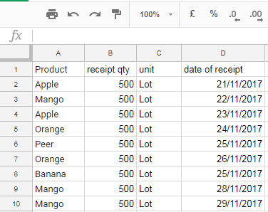
The following sample data consists of receipts of fruits in equal quantities on various dates. It’s in the format Product, Qty, Unit, and Date of Receipt.

We will count the fruit names in column A and determine how many times each fruit repeats in the column. This will indicate the number of lots you received.
Formula:
=QUERY(A1:A, "SELECT A, COUNT (A) WHERE A IS NOT NULL GROUP BY A", 1)When using this formula, you should replace 1 in the last part of the formula with 0 if you don’t have a header at the top of the column.
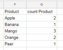
When you apply the above QUERY formula, you will get the following result:

From this, we can find how many times each value repeats in a column. For example, we can see the product Apple repeats twice, Banana once, etc.
The formula follows the syntax QUERY(data, query, [headers]).
Where:
data:A1:A– the column that contains the values to count for occurrences of each value.query:"SELECT A, COUNT(A) WHERE A IS NOT NULL GROUP BY A"– selects and counts column A, filtering out blank rows and grouping by unique values.header:1– the number of header rows.
Two Alternatives to Count How Many Times Each Value Repeats in a Column
I have two interesting combinations to replace the above formula. Both alternatives are worth trying.
1. UNIQUE + COUNTIF
In this method, we will use the UNIQUE function to get the distinct values in column A and COUNTIF to get the count of those values.
Formula:
=ArrayFormula(
   LET(
      val, TOCOL(UNIQUE(A2:A), 1),
      HSTACK(val, COUNTIF(A2:A, val))
   )
)
Formula Explanation:
UNIQUE(A2:A): Returns the distinct values.TOCOL(…, 1): Removes empty cells from the distinct values, if any.- The LET function assigns the name ‘val’ to the above result.
COUNTIF(A2:A, val): Returns the count of ‘val’ in the range A2:A.HSTACK(val, …): Horizontally stacks the ‘val’ with the count results.
The COUNTIF function requires ARRAYFORMULA when counting multiple criteria, here ‘val’ in a range.
Similar to QUERY, this also returns how many times each value repeats in a column. This has one advantage over the QUERY solution: it won’t sort the values in column A.
2. SORTN + COUNTIF
In this approach, we will use the COUNTIF function to count the values in A2:A and SORTN to get the distinct rows.
Formula:
=LET(
   val, TOCOL(A2:A, 1),
   SORTN(HSTACK(val, COUNTIF(val, val)), 9^9, 2, 1, 1)
)
Formula Explanation:
TOCOL(A2:A, 1): Removes empty cells in A2:A.- The LET function assigns the name ‘val’ to this output.
COUNTIF(val, val): Returns the count of values against those values.HSTACK(val, …): Horizontally stacks the ‘val’ with the above output.SORTN(…, 9^9, 2, 1, 1): Returns 9^9 rows, removing duplicates and sorting the ‘val’ in ascending order.
Here the COUNTIF does not require ARRAYFORMULA since the SORTN function acts as an array function.
You can use this to return how many times each value repeats in a column, similar to QUERY.


Is there any formula available?
If I have a column (column A) of unique values data, and a second column (column E) with some values taken from the unique values and repeating again and again, I want to count the repeating values and see how many times each value repeats in column E.
Hi Khalid,
You can use this COUNTIF formula with ARRAYFORMULA:
=ARRAYFORMULA(COUNTIF(E2:E12, A2:A5))Adjust the range references as per your original ranges in the sheet.
I hope this helps!
How would you limit your results to only display the data that actually have duplicates, then their total number of duplicates? (display line items only if the results = 2 or greater)
Hi, Eli,
Use an outer Query as follows.
=query(your_formula_here,"Select * where Col2 >1")Thank you for the great write-up!
Question: how do I preserve the original length of the dataset and add a column of # of occurrences?
Hi, Sunny,
Dataset: A2:A
If so, empty B2:B and insert the following COUNTIF Array Formula in B2.
=ArrayFormula(if(A2:A="",,countif(A2:A,A2:A)))So I need to do something like this but haven’t been able to work it out yet.
I have two date columns in my source data table (received date, complete date).
I would like to create a Query that displays the results as col 1: date, col 2: count of received, col 3: count of complete. Any suggestions? Thx
Hi, Jonny,
You can try this for the range A2:B (A – received, B – completed)
=query(A1:B,"Select A,B,count(A),count(B) where A is not null group by A,B")It returns a four-column Array. So empty D1:G and insert it in cell D1.
That works great!!!!! How do I expend it to count items in multiple columns?
Hi, Hedy T,
I can explain if you share a sample sheet in your comment reply. The link won’t be published.
Syntax has changed on Google Sheets. Use ; instead , … Here the working one:
=QUERY(A2:N1500;"Select A, count (A) WHERE I = TRUE group by A ORDER BY count (A) DESC"; 1)Hi, Aruxandei George Bogdan,
The syntax is different in EU countries and others. But you can control that using the Spreadsheets settings under the File menu.
How to Change a Non-Regional Google Sheets Formula