How to filter rows in a table if the search key is present in any cell in that table in Google Sheets?
Filter rows irrespective of the search key column in that rows in Google Sheets. In other words that is the topic of this post.
In a multi-column dataset, for example, a spare parts requirements table with the part number in one column and part description in another column we can use this type of filter.
Here is my spare parts requirement table and let’s see how the above filtering works.
Sheet Name: Requirement
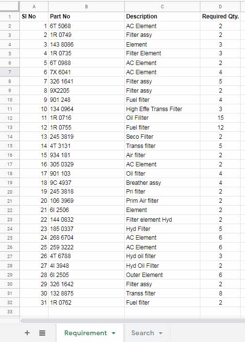
My search key may be the description “Fuel Filter”, part of the description “Filter”, part number starting with “6T” or part number “6T 5068”.
I want to filter the rows in the spare parts requirement table irrespective of the search key present column in that table.
Sheet Name: Search
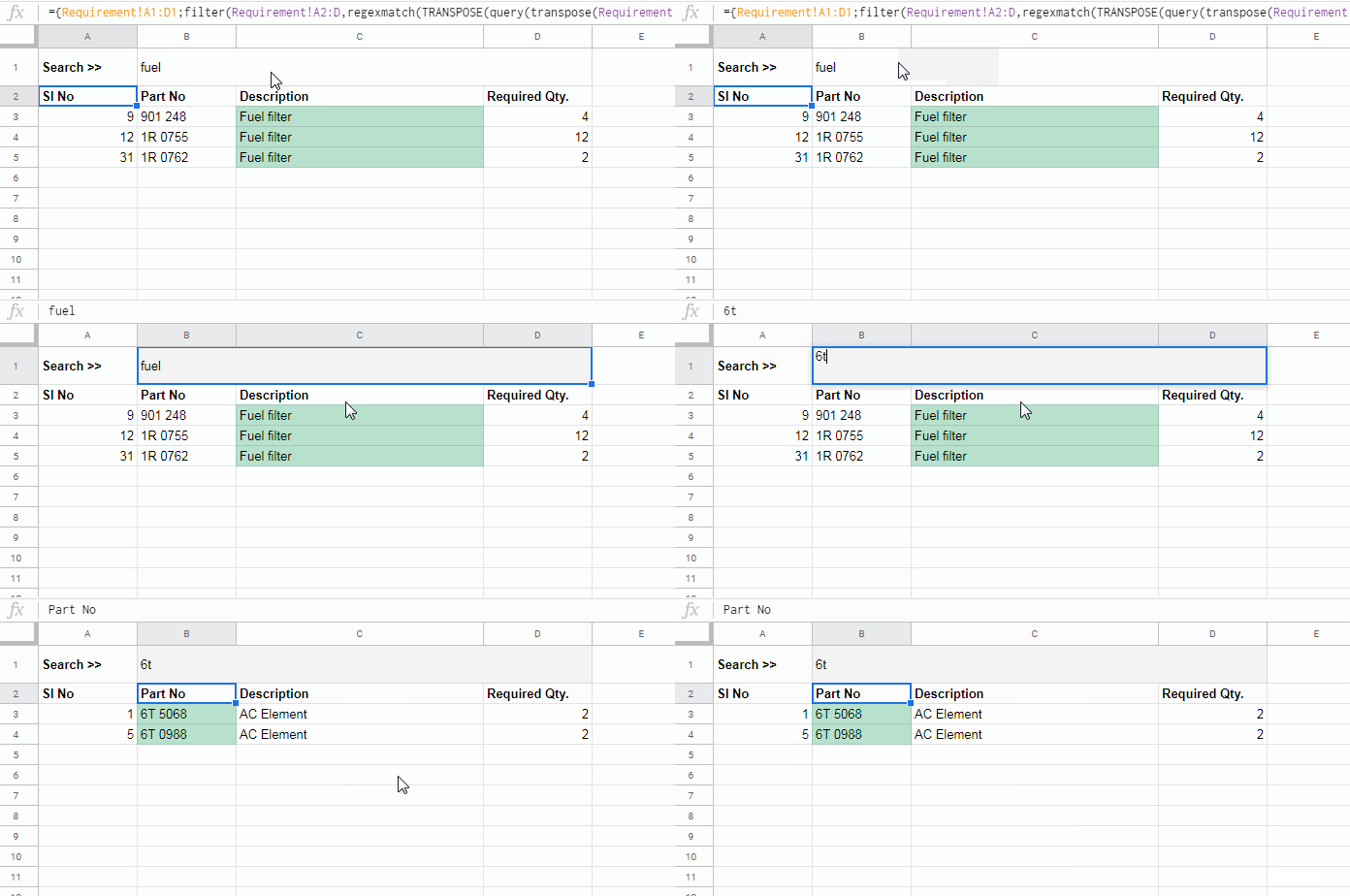
To filter rows if the search key is present in any cell in that rows as above in Google Sheets, we can use the Filter function.
Query and Regexmatch are the other two functions in use. This is not a complex formula and you can learn the use quickly.
How to Filter Rows if the Search Key is Present in Any Cell in Google Sheets
Note: You can find 3-4 formulas below (in different steps). Please note that all the formulas are in “Search” sheet.
I hope you have already gone through the example. In that I have filtered two search keys.
The first time the search key to filter the spare parts is the “fuel” which is in the third column, i.e. Requirement!C1:C, of the spare parts table.
The second time the search key is “6t” which is in the second column, i.e. Requirement!B1:B, of the spare parts table. As you can see I didn’t make any changes in the filter formula in cell A2.
In a normal filter, we must change the “condtion1” column reference to achieve the same.
Syntax: FILTER(range, condition1, [condition2, …])
For example, to filter the table based on the search key “fuel” in cell B1, we can use the below formula in cell A2.
=filter(Requirement!A2:D,regexmatch(Requirement!C2:C,"(?i)"&B1))If the search key is “6t” then the formula must be as follows.
=filter(Requirement!A2:D,regexmatch(Requirement!B2:B,"(?i)"&B1))This is because of the search key column changes in the source table. But we can achieve the same without modifying the formula!
Let’s see how to filter rows when you are unsure about the search key present column in the source table in Google Sheets.
Similar: Regexmatch in Filter Criteria in Google Sheets.
Please follow the below steps.
Query to Format the Dataset (Table) for Filter
To filter rows irrespective of the search key column in those rows, we must format the data using Query. This is the key part.
Assume the sample data is in the “Requirement” sheet and the search key is in the “Search” sheet (two sheets within the same file).
Let’s format the table. First see this Query function syntax.
Syntax: QUERY(data, query, [headers])When writing the Query formula use only the arguments ‘data’ and ‘headers’. We can use an arbitrary number like 1000 as the header.
That means all the 1000 rows used in the ‘data’ are the header rows. This will prompt the Query to combine all the rows to a single row as a header.
This I’ve detailed in my earlier post here – The Flexible Array Formula to Join Columns in Google Sheets.
Instead of 1000 as the query ‘header’ use the count of the total number of rows in your “Requirement” sheet or use 9^9 which is equal to;
Formula: =9^9
Result: 387420489 (an arbitrarily large number)
To properly format the data, here we need to use a series of TRANSPOSE with Query. Here is the syntax to follow to format the table in ‘Requirement’.
=transpose(query(transpose(data),,[header]))Formula # 1 and Output (in ‘Search’ Sheet):
=transpose(query(transpose(Requirement!A2:D),,9^9))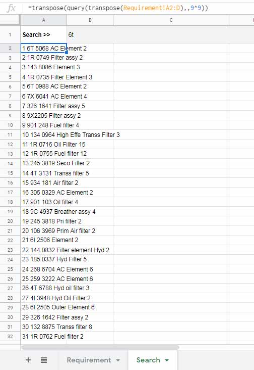
Partial Case Insensitive Match Using Regexmatch in a Query Formatted Data
Here is the second step in the formula to filter rows in a table if the search key is present in any cell in that table in Google Sheets.
I have already linked above a tutorial related to the use of Regexmatch in Filter. If you have no time to check that, don’t worry. I’ll explain the relevant part here.
We can use Regexmatch as below to do a partial and case insensitive match.
For example, cell A2 contains the string “1 6T 5068”. In cell B1 I have the substring to match, which is “6t”.
=REGEXMATCH(A2,"(?i)"&B1)The above Regexmatch will return TRUE. If we want to match the search key in a range, for example, A2:A, use it as below.
Formula # 2:
=ArrayFormula(REGEXMATCH(A2:A,"(?i)"&B1))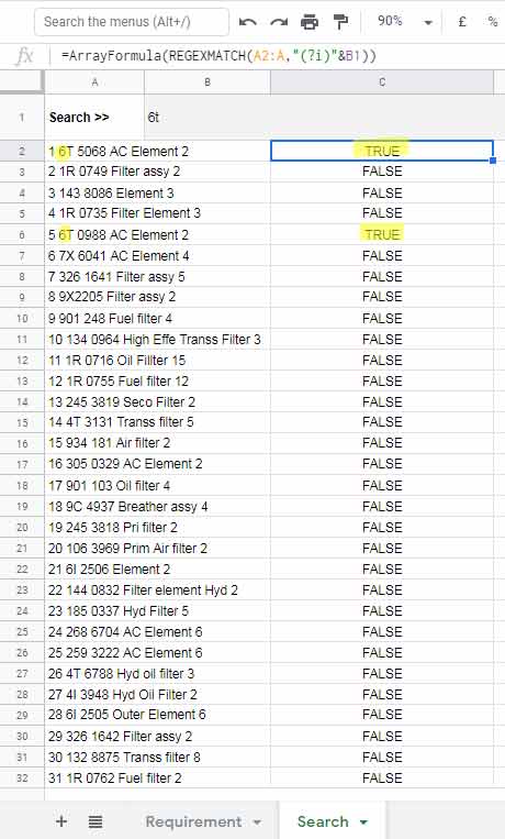
In the next step, I’ll use the above two formulas (formula # 1 and formula # 2) as the ‘condition1’ to filter rows irrespective of the search key column in Google Sheets.
Now let’s replace A2:A in the just above formula with the Query formula, which is in cell A2, itself.
Formula # 3:
=ArrayFormula(REGEXMATCH(transpose(query(transpose(Requirement!A2:D),,9^9)),"(?i)"&B1))Then delete the Query in cell A2.
Final Formula to Filter Rows When the Search Key is Present in Any Cell
Generic Formula:
=filter(Requirement!A2:D,formula_3)In cell A2, based on the generic formula, use the below formula. Then delete the formula in cell C2.
=filter(Requirement!A2:D,regexmatch(TRANSPOSE(query(transpose(Requirement!A2:D),,9^9)),"(?i)"&B1))The above is the formula to filter rows if the search key is present in any cell in Google Sheets.
Finally, click on cell B1 and format it as “Text (Format > Number > Plain text). Otherwise, you may face issues when the search key is number or date.
That’s all. Enjoy!

