How to Filter the Next Row Based on Filter Criteria in Google Sheets

Sometimes you need to grab the next row after a criteria match in Google Sheets—for example, to pull the details that follow a certain label or category.

Sounds simple, right? Well… it’s not always straightforward — especially if your data isn’t in a neat “database” style layout.

Table of Contents

Why This Problem Happens

When your sheet is perfectly structured, filtering is easy.

Example: Properly arranged data

desc	value
supply	1500
purchase	1000

Here, you can just filter the value column for supply or purchase and you’re done.

But sometimes, your sheet looks more like this:

Example: Improperly arranged data

desc and value
supply
1500
purchase
1000

Now things get messy. Your “value” isn’t on the same row as your “desc” — it’s on the next row down. A regular filter won’t work here.

A Real-World Example

Here’s a billing break-up table. Each item (like “Cable” or “Panels”) has several activities, each with a percentage of payment to be released.

Goal: Find the Installation percentage for Panels.

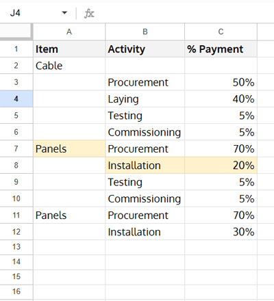
Sample data to filter next row after criteria in Google Sheets

So:

Criteria row = Panels
Target row = the next row (Installation)

The Formula That Does It

Let’s say your data is in A1:C.

Here’s how you can grab the row right after your match:

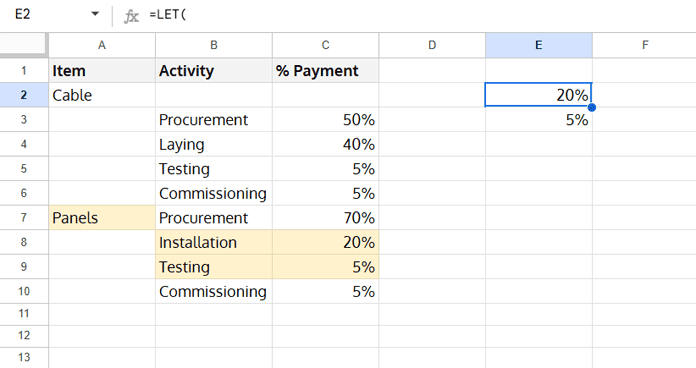
=LET(
   cr, FILTER(ROW(A1:A), A1:A="Panels"),
   nr, {cr+1},
   FILTER(C1:C, XMATCH(ROW(A1:A), nr))
)

Breaking It Down

cr → FILTER(ROW(A1:A), A1:A="Panels")
Finds the row number where Panels appears.
nr → {cr+1}
Adds 1 to that row number to get the next row.
FILTER(C1:C, XMATCH(ROW(A1:A), nr))
Looks up that next row number and pulls the value from column C.

What If You Want More Rows?

Want the next two rows instead of one? Just tweak the {cr+1} part like this:

=LET(
   cr, FILTER(ROW(A1:A), A1:A="Panels"),
   nr, {cr+1; cr+2},
   FILTER(C1:C, XMATCH(ROW(A1:A), nr))
)

That {cr+1; cr+2} means “give me the row after and the one after that.”

Google Sheets formula output showing next row after criteria

You can keep adding more if needed.

What If the Criteria Appears More Than Once?

If you want to filter the next row after a criteria match in Google Sheets only for the first occurrence, simply stick with the formula above.

If you want the next row for all rows matching the filter criteria, you just need to make one change:

Wrap {cr+1} (next row) or {cr+1; cr+2} (next two rows) with the ARRAYFORMULA function, like this:

ARRAYFORMULA({cr+1})

ARRAYFORMULA({cr+1; cr+2})

Why Not Just Use OFFSET?

OFFSET can do something similar, but this LET + FILTER + XMATCH approach is:

Dynamic — no hardcoded row numbers
Stable — won’t break when you add/remove rows
Readable — easier to follow than a long OFFSET formula
Flexible with multiple matches — easily adapts to return rows after every matching criteria, not just the first one