Filter Items Unique to Groups in Google Sheets

In this tutorial, we’ll learn how to filter items unique to groups in Google Sheets.

Whether you’re working with employee names, product codes, or tasks grouped by categories, this method will help you find values that appear only within a single group or category.

Formula to Filter Items Unique to Groups in Google Sheets

=LET(
   unqgr, CHOOSECOLS(SORTN(data, 9^9, 2, 1, 1, 2, 1, 3, 1), 2), 
   unq, UNIQUE(CHOOSECOLS(data, 2)), 
   rc, ARRAYFORMULA(COUNTIF(unqgr, unq)), 
   FILTER(UNQ, rc=1)
)

When you use this formula, replace data with your actual range reference.

Example: Filtering Names Unique to Groups

Assume you are managing multiple projects, and an employee assigned to one project may also be involved in others.

You want to find employees who are assigned to only one project, so you can allocate them elsewhere in case of an emergency.

In this example, we filter the names of employees assigned to only one project.

Sample Data

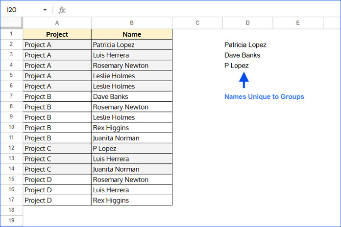
Example of Filtering Names Unique to Groups in Google Sheets

This data consists of projects in column A (groups) and employee names in column B (items).

Apply the Formula

You can use the following formula in cell D2 to filter names unique to groups:

=LET(
   unqgr, CHOOSECOLS(SORTN(A2:B, 9^9, 2, 1, 1, 2, 1, 3, 1), 2), 
   unq, UNIQUE(CHOOSECOLS(A2:B, 2)), 
   rc, ARRAYFORMULA(COUNTIF(unqgr, unq)), 
   FILTER(UNQ, rc=1)
)

The formula will return the following names:

Patricia Lopez
Dave Banks
P Lopez

How the Formula Filters Items Unique to Groups in Google Sheets

Formula Explanation:

unqgr
CHOOSECOLS(SORTN(A2:B, 9^9, 2, 1, 1, 2, 1, 3, 1), 2)
Returns the list of unique names within each project.
SORTN removes duplicate rows, and CHOOSECOLS extracts only the names column.
unq
UNIQUE(CHOOSECOLS(A2:B, 2))
Returns all unique names from the “items” column (column B) in the dataset.
rc
ARRAYFORMULA(COUNTIF(unqgr, unq))
Counts how many times each unique name appears across the projects after removing duplicate names within the same project.
FILTER(unq, rc=1)
Filters and returns only the names whose occurrence count is exactly 1 — meaning they appear in only one project.

This is how you can filter items unique to groups in Google Sheets, whether you’re working with employee names, product codes, or other items grouped by categories.

Note:

These formulas do not require your data to be sorted by groups. They will work even if the entries are mixed or unordered.

Additional Tip: Highlight Items Unique to Groups

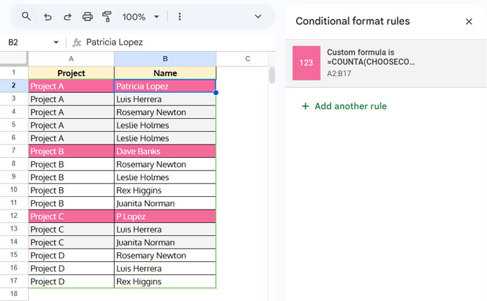
If you don’t want to filter items unique to groups but highlight them instead, you can use this formula in Conditional Formatting:

=COUNTA(CHOOSECOLS(UNIQUE(FILTER($A$2:$B, $B$2:$B=$B2)), 2))=1

This formula checks if a name appears in only one project. It filters the dataset to find all projects associated with the current name ($B2), removes duplicates, and counts how many unique projects are linked to it. The rule highlights the name if the count is 1.

Here’s how to set it up:

Select the range (A2:A, B2:B, or A2:B) depending on what you want to highlight.
Go to Format > Conditional formatting.
Under “Format cells if,” choose Custom formula is.
Enter the above formula.
Set your formatting style and click Done.

This will highlight names unique to projects.

An advantage of this method:

You can then use Data > Create a filter > Filter by color to easily filter items unique to categories.