


Filter rows and filter groups are two different things. First, understand the difference then you can learn how to filter groups which match at least one condition/criterion in Google Sheets.
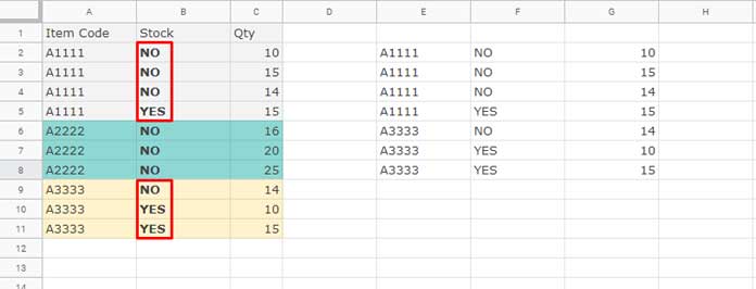
My data, sample data only, contains three columns and the column names are “Item Code”, “Stock”, and “Qty”.
First I am going to filter rows. Here is the sample dataset that I am going to use throughout this tutorial.
| A | B | C | |
| 1 | Item Code | Stock | Qty |
| 2 | A1111 | NO | 10 |
| 3 | A1111 | NO | 15 |
| 4 | A1111 | NO | 14 |
| 5 | A1111 | YES | 15 |
| 6 | A2222 | NO | 16 |
| 7 | A2222 | NO | 20 |
| 8 | A2222 | NO | 25 |
| 10 | A3333 | NO | 14 |
| 11 | A3333 | YES | 10 |
| 12 | A3333 | YES | 15 |
Of course, you can use an entirely different dataset with as many numbers of rows and columns that you want. But first, follow the above one.
Here is the FILTER formula to filter all the rows that contain “YES”, which is our condition/criterion, in column B.
=filter(A2:C,B2:B="YES")This filter formula would filter row # 5, 11, and 12 from the above dataset. See the “Stock” column 2 to find the reason. What about filter groups then?
It’s actually about filtering any one (or more than one) group as below.
=filter(A2:C,A2:A="A2222")The above filter formula filters the row # 6, 7, and 8. Hope you could understand the difference between filter rows and filter groups in Google Sheets.
How to Filter Groups That Match at Least One Condition/Criterion in Sheets
In filtering groups that match at least one condition, we are not going to filter any particular group as above (second formula above). Instead, we are filtering all the groups that match at least one condition in a second column. Here that condition is “YES” in column B.
Here the groups are “A1111”, “A2222”, and “A3333”. In these three groups, the first and the last groups have at least one matching condition, i.e. “Yes”, in column B.
My filter formula, which is a combination formula, in cell E1 filters the said matching groups.
Google Sheets Formula to Filter Group of Rows That Match a Criterion:
I have used a Vlookup and Filter combination to filter groups as above. In cell E2, I have the below combo formula.
=filter(A2:C,IFNA(vlookup(A2:A,filter(A2:A,B2:B="YES"),1,0))<>"")I will definitely explain how this formula filters groups based on matching one criterion. There are three steps involved.
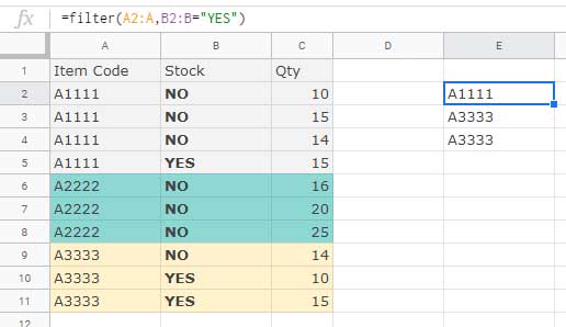
Step # 1: Filter Rows (Only the First Column) that Match One Criterion
In the above master formula, please see the Filter formula inside the Vlookup. It’s as below.
filter(A2:A,B2:B="YES")It filters the rows and returns the first column if the column B value is “YES”.
Step # 2: Vlookup Groups Which Match at Least One Condition in Google Sheets
The above Filter formula helps us to Vlookup groups which match at least one criterion.
Formula:
=ArrayFormula(IFNA(vlookup(A2:A,filter(A2:A,B2:B="YES"),1,0)))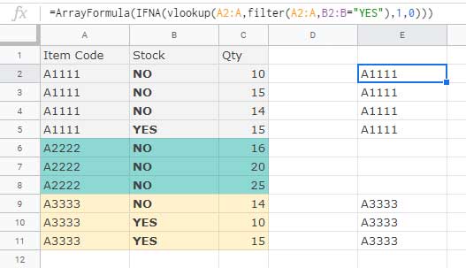
Explanation:
The Vlookup formula searches the keys (groups) which are in A2:A in the first column of the filtered (step # 1 formula) output.
VLOOKUP(search_key, range, index, [is_sorted])I mean the ‘search_keys’ are in A2:A, and the ‘range’ is the step # 1 formula. The ‘index’ column (Vlookup output column from the ‘range’) is 1.
Since the filter output (‘range’) misses the key “A2222”, Vlookup will return N/A in row # 6, 7, and 8 which I have removed using the IFNA outside the Vlookup.
Note: Earlier I was using IFERROR instead of IFNA. IFNA is a ‘new’ function (I have noticed it quite recently) in Sheets. I recommend you to use IFNA instead of IFERROR in Vlookup as we simply want to remove N/A errors.
Step # 3: Final Filter+Vlookup+Filter Combo Formula
To filter groups which match at least one condition, simply filter the range A1:C using the Formula # 2 output as the criteria. It must be used like this. See the <>"" at the last part of this formula.
IFNA(vlookup(A2:A,filter(A2:A,B2:B="YES"),1,0))<>""That means filter all the rows, wherever the formula # 2 output isn’t blank.
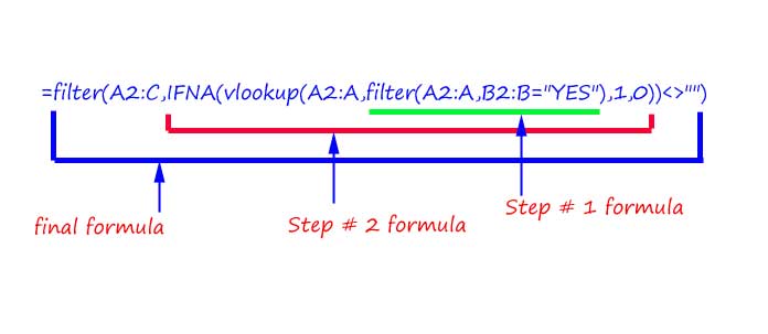
I hope the above illustration will give you a clear idea about how I have combined the formulas. Enjoy!