Google Sheets offers many tools to summarize and analyze data, but Pivot Tables are one of the most powerful options. Did you know you can take your analysis even further by applying a filter by total in a pivot table?

For example, you may want to filter by total sales, displaying only products or salespeople with sales above a certain threshold (e.g., $5000). Another example is filtering schools based on participation, showing only those that have participated in at least three events.

In this guide, you’ll learn how to filter by total in a pivot table in Google Sheets using a custom formula within the filter field, with step-by-step examples.

Example 1: Filter by Total Sales in a Pivot Table

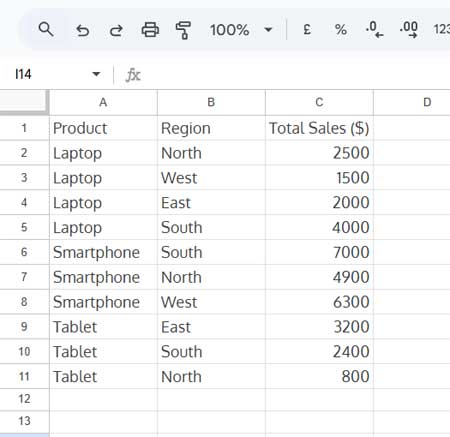
In this example, we have Product, Region, and Total Sales in columns A, B, and C, respectively. Let’s create a pivot table grouped by Product and Region (Row Grouping) with Total Sales as the value.

The goal is to filter the pivot table to show only products with total sales greater than $10,000.

Creating the Pivot Table

1. Select the data range A1:C and go to Insert > Pivot Table.
2. In the popup window, choose “Existing Sheet,” select cell E1, and click Create. This will open the pivot table editor.
3. Set up the pivot table with:
   • Rows: Product, then Region (you can also select only one field if needed).
   • Values: Total Sales ($) (summarized by SUM).

This setup generates the following pivot table:

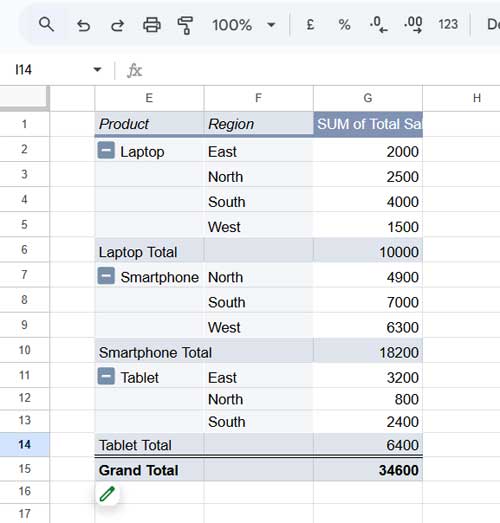
Since Tablet has total sales less than $10,000, we want to filter it out.

Custom Formula to Filter by Total in Pivot Table

To filter products based on total sales, we’ll apply the following custom formula:

=SUMIF(A:A, Product, C:C)>=10000

Formula Breakdown

• A:A: The column containing product names.
• Product: The current product being evaluated in the pivot table.
• C:C: The column containing total sales.

SUMIF returns the total sales for each product, and the filter retains only those where total sales >= 10,000.

We specify entire columns (A:A and C:C) to accommodate future data.

Applying the Filter

1. Open the Pivot Table Editor by clicking the pencil icon, then click Filters.
2. Select Product as the filter field.
3. Click the drop-down and choose Filter by Condition > Custom Formula Is.
4. Copy-paste the formula: =SUMIF(A:A, Product, C:C)>=10000
5. Click OK.

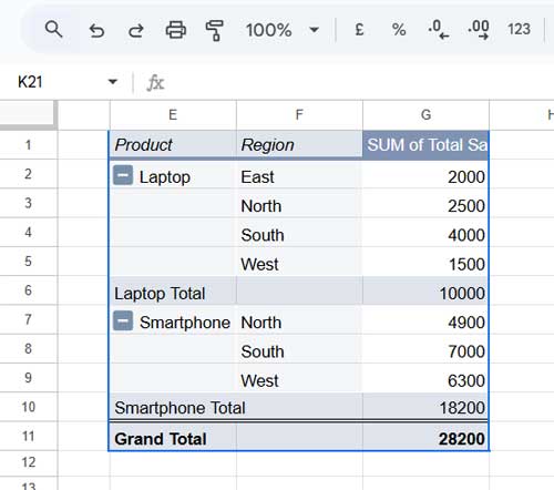
This will filter the pivot table, keeping only products where total sales >= $10,000.

How Does This Filter Work?

The SUMIF formula calculates the total sales per product. If the total sales for a product meet or exceed $10,000, the pivot table retains that row; otherwise, it is filtered out.

Example 2: Filter by Number of Events Participated

Now, let’s see another example where we filter a pivot table based on the number of events each school has participated in.

Dataset

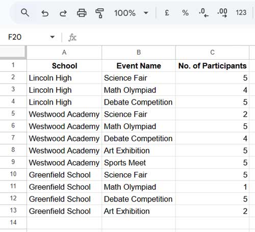
We want to filter out schools that have participated in fewer than 3 events.

Creating the Pivot Table

1. Select the data range and go to Insert > Pivot Table.
2. Set up the pivot table with:
   • Rows: School, then Event Name.
   • Values: School (summarized by COUNTA to count events per school).

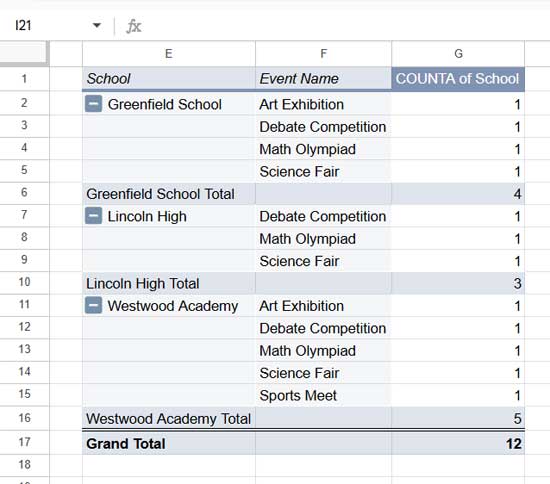
Custom Formula to Filter by Event Participation

To filter schools based on the number of events they participated in, apply the following formula:

=COUNTIF(A:A, School)>3

Formula Breakdown

• A:A: The column containing school names.
• School: The current school being evaluated in the pivot table.

COUNTIF counts the number of events for each school. If the total is greater than 3, the pivot table retains that row.

Applying the Filter

1. Open the Pivot Table Editor and click Filters.
2. Select School as the filter field.
3. Click the drop-down and choose Filter by Condition > Custom Formula Is.
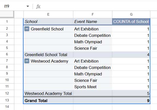
4. Copy-paste the formula: =COUNTIF(A:A, School)>3
5. Click OK.

This will filter out schools that participated in fewer than 3 events.

Conclusion

We explored two different ways to filter by total in a pivot table in Google Sheets:

1. Filtering by total sales using SUMIF.
2. Filtering by total count of events using COUNTIF.

Both methods use custom formulas within the pivot table filter field, making them highly flexible. You can adapt these techniques for other scenarios, such as filtering by revenue, order count, or attendance.

Tip: Always use open-ended column references like A:A to ensure your filter works dynamically when new data is added.

If you have any questions, feel free to ask in the comments below!

Sample Sheets

Resources

• How to Filter Top 10 Items in Google Sheets Pivot Table
• Filter Top 3 Values in Each Group in Pivot Table – Google Sheets
• Filter Multiple Values in Pivot Table in Google Sheets
• How to Add a Running Total in Pivot Table in Google Sheets
• How to Sort Pivot Table Grand Total Columns in Google Sheets
• Adding Calculated Fields in Pivot Table in Google Sheets