


We must use parentheses to define explicit precedence when using logical operators AND, OR, and NOT in Google Sheets Query.
When using more than one logical operator in Query to join multiple conditions, we must use parentheses to define explicit precedence.
Otherwise, the formula won’t return the correct information that we want.
Here my sample data contains eight records that spread across seven columns. I want to retrieve the item codes (column A) based on the below conditions.
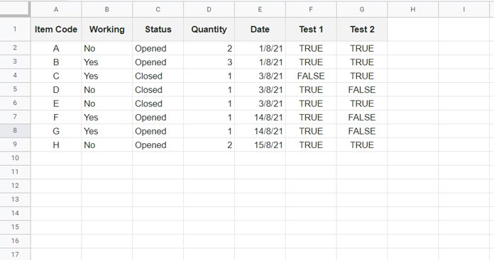
Filter records if:
1. Either column B = “Yes” or column C = “Opened” (Condition 1 [highlighted in Cyan color on the image below])
And;
2. F = TRUE (Condition 2 [highlighted in Green])
3. G = TRUE (Condition 3 [highlighted in Yellow])
Here is the correct formula that will return the required output.
=QUERY(A1:G, "select A where (B='Yes' or C='Opened') and F=TRUE and G=TRUE")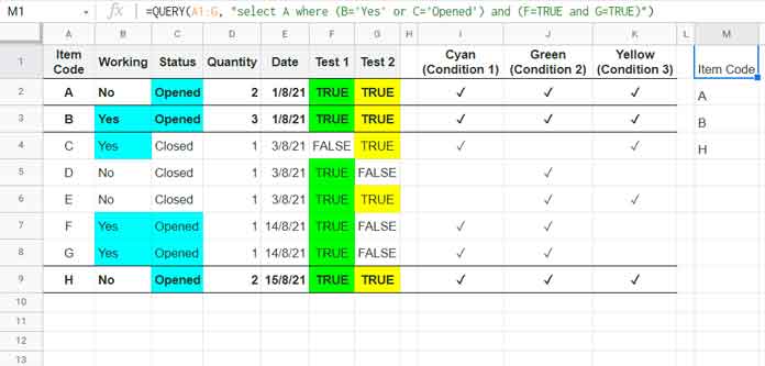
In the above example, all three conditions are met in rows 2, 3, and 9.
The parentheses around the OR operators are important.
If we want, we can use them around the AND also as show in the image above.
Here is an alternative formula that will return the same records:
=QUERY(A1:G, "select A where F=TRUE and G=TRUE and (B='Yes' or C='Opened')")What Happens When I Do Not Define Explicit Precedence in Google Sheets Query?
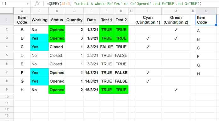
Assume we have removed the parenthesis around the OR operators as below.
=QUERY(A1:G, "select A where B='Yes' or C='Opened' and F=TRUE and G=TRUE")It will produce a different result because the query is evaluated in the following order.
Filter records if:
1. Column B = “Yes”
Or;
2. Column C = “Opened,” and Column F = TRUE, and Column G = TRUE.
In the first example above, you can find an “alternative formula”. In that formula also, I have used parenthesis to define explicit precedence.
What happens when we remove them?
Formula:
=QUERY(A1:G, "select A where F=TRUE and G=TRUE and B='Yes' or C='Opened'")This query will evaluate in the following order:
Filter records if:
1. Column F = TRUE, and Column G = TRUE, and Column B = “Yes”
Or;
2. Column C = “Opened”.
So the result will be the item codes in rows 2, 3, 4, 7, 8, and 9.
That’s all. Thanks for the stay. Enjoy!
Query Resources
- How to Use Date Criteria in Query Function in Google Sheets.
- How to Use LIKE String Operator in Google Sheets Query.
- CONTAINS Substring Match in Google Sheets Query for Partial Match.
- Matches Regular Expression Match in Google Sheets Query.
- How to Use Not Equal to in Query in Google Sheets.
- How to Use Arithmetic Operators in Query in Google Sheets.
- Starts with and Not Starts with Prefix Match in Query.
- Ends with and Not Ends with Suffix Match in Query.
Hi Prashanth! Thank you for all those great articles (: I’m so happy each time I google something I’m stuck with and find your website with the exact answer.
I’ve tried to replicate the ‘explicit precedence’ using date criteria by excluding a date range but couldn’t make the formula returns the correct results.
Any idea?
Thanks!
Hi, Dimitri Leroux,
I’m glad to hear that you find my tutorials worthy.
Regarding the issue with your formula, please include the URL of that sheet in your reply below. I won’t publish that comment.
A sample sheet URL will also do.
Here is the public link:
— removed by admin —
I changed the data to make it looks simple 🙂 Thank you so much for looking at it!
Hi, Dimitri Leroux,
I’ve inserted the formula in your sheet.
You were trying to sum the last 30 days’ data that excluding a certain date range.
To exclude the date range, I have used the NOT operator.
Hi Prashanth, just realized your help with the sheet! Thanks so much, nice way around to make it matches the result again.
I also noticed your changes with:
– to_date(index(split( … instead of … to_date(datevalue(left(
– arrayformula(query{ … instead of … query({arrayformula(
Is it because of coding conventions, or it also affects the speed at which the spreadsheet is loaded? (same as putting formula inline)
Hi, Dimitri Leroux,
I don’t think those changes make any speed improvement. I just wrote it that way.