


")


")

")
")
 in Excel & Google Sheets")


To obtain a dynamic sum column (sum_range argument) in SUMIF, we can utilize the XLOOKUP or INDEX function in Google Sheets.
The XLOOKUP will be useful when looking up the header to find the sum range.
The INDEX will be useful when you use the LET function to assign names or the LAMBDA function to create custom functions.
Regarding the LET or LAMBDA use, you may assign the name ‘data’ to the whole range and extract specific columns in SUMIF using CHOOSECOLS. This may cause the “Argument must be a range” issue. You can resolve this by using OFFSET or INDEX, which we will see in the examples.
Examples of Specifying a Dynamic Sum Column in SUMIF in Google Sheets
We will see examples of this in the following sample sales data, which contains two amount columns: Sales and Returns.
Example 1: Using XLOOKUP in Sum_Range of SUMIF
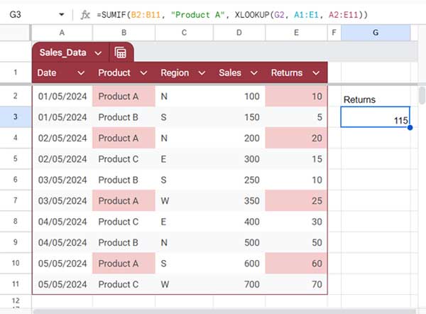
The below formula sums the return amount of “Product A”:
=SUMIF(B2:B11, "Product A", XLOOKUP("Returns", A1:E1, A2:E11))This adheres to the following SUMIF syntax: SUMIF(range, criterion, [sum_range]).
Where:
range: B2:B11 (the column containing the product names which is tested againstcriterion)criterion: “Product A”sum_range:XLOOKUP("Returns", A1:E1, A2:E11)(matches the keyword “Returns” in the header row and returns the values below)
If you replace ‘Returns’ with ‘Sales’, it will output the sum of the ‘Sales’ amount.
This example specifies a dynamic sum column in the SUMIF function. The XLOOKUP function plays a key role by dynamically fetching the sum_range.
Formula with Structured Table Reference:
Our sample data is a range converted to a table, and the table name is Sales_Data. How do I rewrite the above formula with a structured table reference?
As per my table, you should make the following changes to the SUMIF formula:
B2:B11becomesSales_Data[Product]A1:E1becomesCHOOSEROWS(Sales_Data[#ALL], 1)A2:E11becomesSales_Data
Formula:
=SUMIF(Sales_Data[Product], "Product A", XLOOKUP("Returns", CHOOSEROWS(Sales_Data[#ALL], 1), Sales_Data))To learn more about structured table references, please check out: Structured Table References in Formulas in Google Sheets
Example 2: Using INDEX in Sum_Range of SUMIF
In some scenarios, we may be required to specify the column number instead of the range reference in the range and sum_range of SUMIF.
This mostly happens when we use the LET or LAMBDA functions and assign names to ranges. Let’s start with LET.
LET Example:
Please see the following example:
=LET(data, A2:E11, SUMIF(CHOOSECOLS(data, 2), "Product A", INDEX(data, 0, 5)))We have assigned the name “data” to the range A2:E11 using the LET function. The SUMIF arguments are as follows:
range: CHOOSECOLS(data, 2) – selects the second column in the ‘data’.criterion: “Product A”sum_range: INDEX(data, 0, 5) – selects the fifth column in the ‘data’.
In sum_range, we can’t use CHOOSECOLS(data, 5) to specify the fifth column as it will invite the infamous “Argument must be a range” error. So, we have used the INDEX function, which follows the syntax INDEX(reference, [row], [column]).
Where the reference is ‘data’, the row is 0 (return all rows), and the column is 5 (return the 5th column).
You can also use OFFSET (OFFSET(Data, 0, 4,,1)) instead of INDEX.
This is another example of a dynamic sum column in the Google Sheets SUMIF function.
LAMBDA Example:
When writing custom functions using LAMBDA, we prefer to use as few arguments as possible.
Let’s create a custom function out of the above SUMIF formula that uses dynamic column references in the range and sum_range.
=LAMBDA(range, SUMIF(CHOOSECOLS(range, 2), "Product A", INDEX(range, 0, 5)))(A2:E11)The formula expressions in this and the LET function are the same, which is the SUMIF function. The only difference is in how we assign the name to the range.
In LET, we specify the name, associated value_expression (range reference), and then the formula_expression follows.
Whereas in the LAMBDA function, you specify the name and formula expression. After closing the formula expression, you specify the range reference (function call) separately.
Conclusion
Here are a few related tutorials.