Many users rely on a helper column to mark and delete every nth row in Google Sheets. However, you can do this without a helper column by using the “Create a filter” option in the Data menu.
In this guide, I’ll show you how to delete every second, third, fourth, or nth row in Google Sheets using filters—no scripting or AI required.
Why Delete Every Nth Row in Google Sheets?
I needed to delete every 4th row in one of my tables because those rows contained labels that interfered with other spreadsheet formulas like QUERY. Having labels mixed with numeric data creates mixed content, which can cause issues in formulas that expect uniform data types.
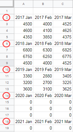
If you’re unfamiliar with mixed content data, see the example below. Labels appear at every 4th row, making the entire column a mixed data type.

How to Filter and Delete Every Nth Row in Google Sheets
I’ll first demonstrate how to filter and delete every 4th row. Then, I’ll show how to modify the formula to delete any nth row.
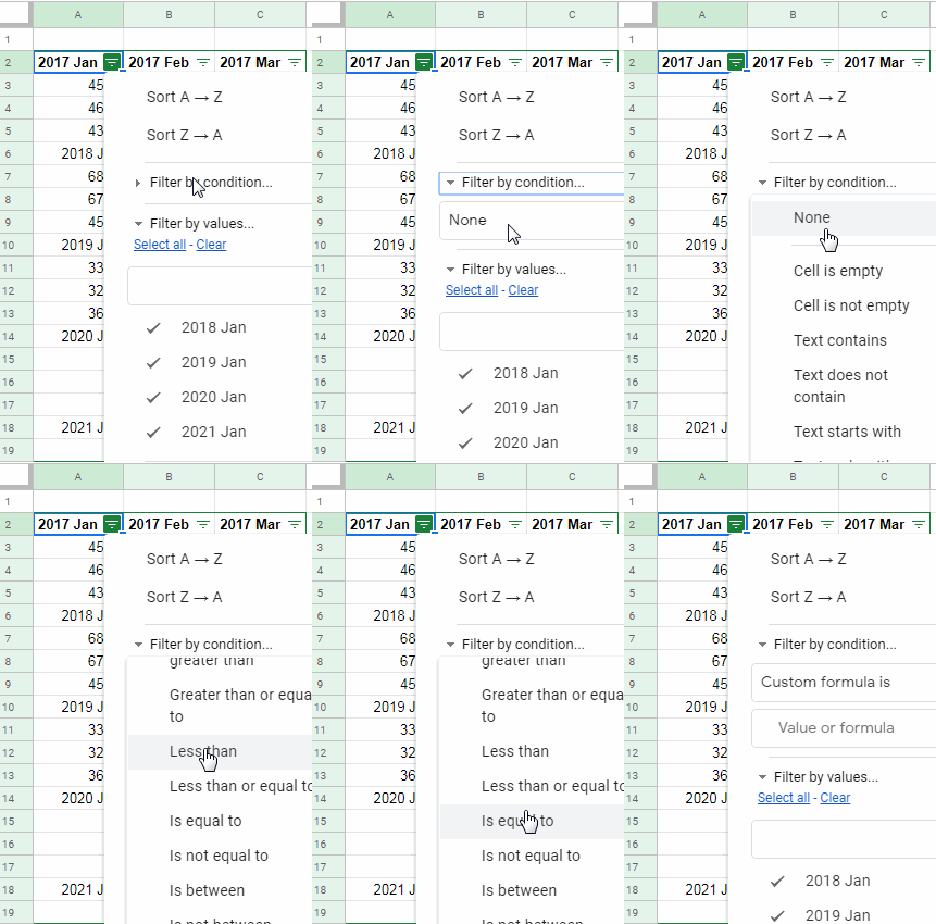
1. Set Up Filters
- Click on the first cell in your data range (e.g.,
A2). - Go to the Data menu and select Create a filter.
- Click the filter icon in the first column (cell
A2). - Select Filter by condition > Custom formula is.

2. Apply a Custom Formula to Filter Every Nth Row
Enter the following MOD formula in the provided field and click OK:
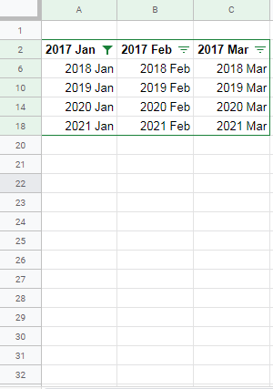
=MOD((ROW(A3)-ROW($A$3)+1), 4)=0This formula filters only the rows that contain labels (every 4th row in this case). You will now see only the selected nth rows in your dataset.

Note: The formula should reference the first data row (e.g., A3) rather than the header row. If your data starts from a different row, adjust the reference accordingly.
3. Delete the Filtered Rows
Select the visible rows:
- To select all filtered rows at once, click on the first visible row number (e.g., row 6), then hold down the Shift key and click the last visible row number (e.g., row 18). This selects all filtered rows in one go.
- To select rows individually, hold down the Ctrl (Cmd on Mac) key and click each row number one by one (e.g., 6, 10, 14, and 18).
Delete the selected rows:
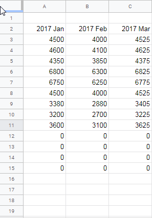
- Right-click on any selected row and choose Delete selected rows.
Turn off the filter:
- Go to the Data menu and click Remove filter, or use the shortcut Alt + D + F.

Modify the Formula to Filter Every Nth Row
To delete a different nth row, modify the formula as follows:
- Delete every 2nd row:
=MOD((ROW(A3)-ROW($A$3)+1), 2)=0- Delete every 3rd row:
=MOD((ROW(A3)-ROW($A$3)+1), 3)=0- Delete every 5th row:
=MOD((ROW(A3)-ROW($A$3)+1), 5)=0The pattern is simple: change the divisor (the number after the comma in MOD) to the nth row number you want to filter.
Summary
To delete every nth row in Google Sheets:
- Apply a filter using the “Create a filter” option in the Data menu.
- Use a custom formula with
MODto filter every nth row. - Select and delete the filtered rows.
This method is efficient and requires no scripting. You can use it to clean up large datasets quickly.
Related Resources
- How to Sum Every Nth Row or Column in Google Sheets
- How to Highlight Every Nth Row or Column in Google Sheets
- How to Copy Every Nth Cell from a Column in Google Sheets
- Select Every Nth Column in Google Sheets Query – Dynamic Formula
- Extract Every Nth Line from Multi-Line Cells in Google Sheets
- Import Every Nth Row in Google Sheets Using Query or Filter (Same File)
- INDEX MATCH Every Nth Column in Google Sheets
- Date Sequence Every Nth Row in Excel (Dynamic Array)


Hello,
Thank you for this!
I was wondering if it is possible to delete every 16th and 17th row. I have two nth rows in my custom filter.
=mod((row (A3)-row($A$3)+1), 16, 17) = 0Would this work?
Hi, Angela,
This may help.
=or(mod((row(A3)-row($A$3)+1),16)=0,mod((ROW(A3)-row($A$3)+1),16)=1)