")


")


")

")
")
 in Excel & Google Sheets")


Google Sheets’ new table feature offers limited options for customizing colors. While you can customize overall table colors, the impact is minimal as it primarily changes something like a theme color.
You can toggle the default alternating colors of a table on and off, but there’s no option to customize them.
If you want to achieve a vibrant look by customizing the alternating colors of a table, here are the step-by-step instructions.
Customizing Alternating Colors of a Google Sheets Table
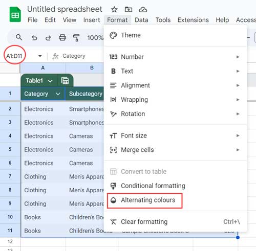
Select the table, including the header row.
Go to the Format menu and click on “Alternating Colors” to open the alternating colors side panel.
Default table styles will be displayed. To customize the alternating colors of the table, navigate to the “Custom Style” section. Ignore the default styles and select your desired alternating colors by clicking the drop-down menus next to “Color1” and “Color2.”

Click “Done.”
How Table Settings Affect the Newly Applied Colors
Two table settings influence the customized alternating table colors:
- Customize Table Colors
- Turn Off Alternating Colors
You can access these options by clicking the drop-down next to the table name in the top-left corner of the table.
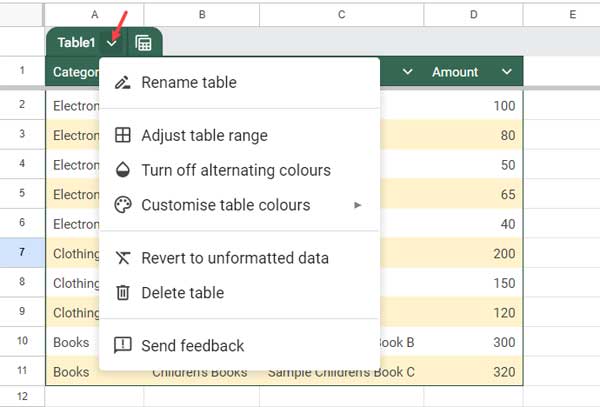
Using the “Customize Table Colors” option allows you to change the theme color of the table without affecting the alternating colors you’ve set. This option is useful for modifying the header background color.
However, turning off alternating colors will impact the customized alternating colors. When you toggle this setting off and then on again, it will revert to the default alternating colors. In such cases, you’ll need to reapply the customization using the steps outlined above.
Adjusting Table Range and the Impact of Customized Alternating Colors
When you add more data in adjacent rows or columns, or manually adjust the table range, the customized alternating colors will expand accordingly. You don’t need to reapply the alternating colors to the newly added range.
As a side note, to manually increase the table range, click the drop-down next to the table name and select the “Adjust table range” option. Enter the desired table range in the window that appears, then click OK.
Resources
Below are some useful resources discussing the new Table feature in Google Sheets. Additionally, I’ve included tutorials related to customizing alternating colors in a range.