


")


")

")
")
 in Excel & Google Sheets")


By default, Google Sheets’ QUERY function does not support defining a custom sort order using the ORDER BY clause. However, there is a workaround! You can first process the data using QUERY and then apply custom sorting with the SORT function. This can all be combined into a single formula using the LET function for convenience.
What Is a Custom Sort Order?
A custom sort order allows you to sort a column in a specific order rather than the default alphabetical or sequential order.
If you’ve processed data using QUERY and want to sort a specific column in a custom order, this approach will help.
Generic Formula
=LET(
   qry, your_query_formula,
   order, ARRAYFORMULA(XMATCH(CHOOSECOLS(qry, sort_column), custom_order)),
   SORT(qry, order, 1)
)
Formula Explanation:
your_query_formula– Your QUERY formula (without custom sorting).sort_column– The column index within the QUERY output that you want to sort.custom_order– An array or range containing the unique values arranged in your preferred order.
Example: Applying Custom Sort Order in QUERY
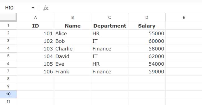
Below is a sample dataset containing Employee ID, Name, Department, and Salary:
Basic QUERY Sorting (Alphabetical Order)
The following QUERY formula selects all rows (excluding empty ones) and sorts by the third column (Department) in ascending order:
=QUERY(A1:D, "SELECT * WHERE Col1 IS NOT NULL ORDER BY Col3 ASC")This results in Finance appearing first, followed by HR and IT (alphabetical order).
Applying a Custom Sort Order
Now, let’s say you want the Department column to be sorted in this custom order: HR → Finance → IT
Here’s how to modify the QUERY formula to apply a custom sort order:
=LET(
   qry, QUERY(A1:D, "SELECT * WHERE Col1 IS NOT NULL ORDER BY Col3 ASC"),
   order, ARRAYFORMULA(XMATCH(CHOOSECOLS(qry, 3), {"Department"; "HR"; "Finance"; "IT"})),
   SORT(qry, order, 1)
)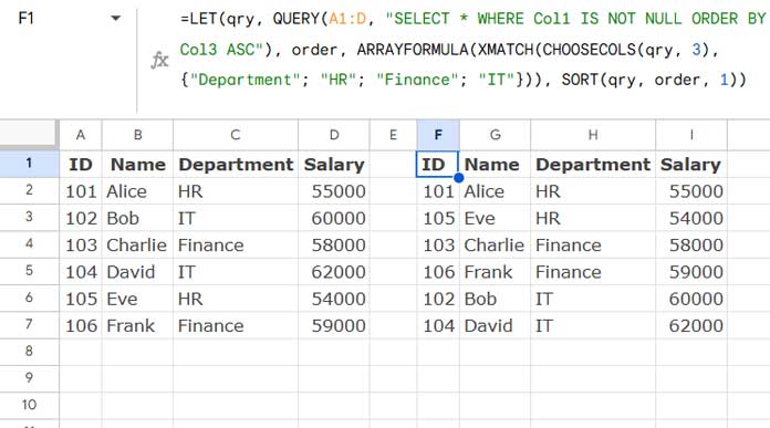
Breakdown of the Formula:
QUERY(A1:D, "SELECT * WHERE Col1 IS NOT NULL"): Fetches data, excluding empty rows.CHOOSECOLS(qry, 3): Extracts the third column (Department) from the QUERY output.XMATCH(CHOOSECOLS(qry, 3), {"Department"; "HR"; "Finance"; "IT"}): Assigns a custom sorting order.SORT(qry, order, 1): Sorts the QUERY results based on the custom order.
Alternative Approach Using Cell References
Instead of manually typing the custom order in the formula, you can enter the sorting values in E1:E4 as follows:
| E |
| Department |
| HR |
| Finance |
| IT |
Now, update the formula to use the range instead:
=LET(
   qry, QUERY(A1:D, "SELECT * WHERE Col1 IS NOT NULL ORDER BY Col3 ASC"),
   order, ARRAYFORMULA(XMATCH(CHOOSECOLS(qry, 3), E1:E4)),
   SORT(qry, order, 1)
)
This makes it easier to update the sort order dynamically.
FAQs
1. What happens if the custom order does not match all values?
If all values in the column do not match the custom order, the QUERY result remains unchanged. If some values match, they will be sorted as per the custom order, while unmatched values appear at the bottom in their default order.
2. What if my QUERY result does not have a header row?
In that case, exclude the header from the custom order array/range.
How did you avoid the following Error Message by not including Col3 in the “Select” portion of your query?
"Error COL_IN_ORDER_MUST_BE_IN_SELECT: 'Col3'"Hi, Dave,
I don’t get that error on my side. Can you share a sample?
Awesome, That’s brilliant.
Just for completeness, why does the ArrayFormula need to be moved to the outside, and what happens if it isn’t placed there?
Thank again – This should allow ordering output by weekdays in proper order!
Hi, Stu,
It won’t make any difference in this case. But make it a practice.
If you have two or more ArrayFormulas in a combination formula, you can remove all that by placing only one ArrayFormula in the front.