If you’re working with data spread across multiple columns in Google Sheets, you may need to count how many unique values appear—either across all columns combined, within each column separately, or by pairing values (such as first and last names).
While Google Sheets offers a built-in COUNTUNIQUE function, it doesn’t directly support all of these use cases—especially when dealing with multiple columns or filtered data.
In this tutorial, I’ll show you how to count unique values in multiple columns in Google Sheets in two main ways:
- Without combining values — to count how many distinct values appear across all columns.
- With combining values — to treat entries like full names across columns as a single unique entity.
Whether you’re managing names, survey answers, or categories, these methods will help you accurately count unique values in multiple columns.
1. Counting Unique Values in Multiple Columns Without Combining
Imagine you’re analyzing responses to the question: “Which programming languages do you use regularly?”
Your dataset (in range A1:D) looks like this:
| Name | Q1 | Q2 | Q3 |
| Ansh | Python | JavaScript | SQL |
| Ben | JavaScript | Java | |
| Ahana | Python | SQL | C++ |
| David | C# | JavaScript | Python |
| Aditi | Java | R |
To count how many unique programming languages were selected across all questions (Q1 to Q3), use the following formula:
=COUNTUNIQUE(TOCOL(B2:D, 3))Explanation:
TOCOL(B2:D, 3)flattens the selected columns into a single column, ignoring empty cells.COUNTUNIQUEthen returns the number of distinct values across all three columns.
This method is ideal when you want to find unique values across multiple columns without combining values from adjacent columns.
2. Counting Unique Values in Multiple Columns With Combining
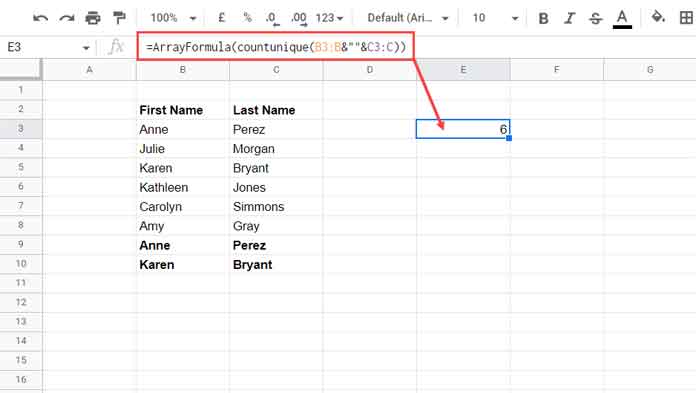
Now let’s say you’re working with first and last names stored in separate columns, and you want to count how many unique full names exist.
Your data might look like this:

To count unique full names (i.e., first + last combined), use:
=ARRAYFORMULA(COUNTUNIQUE(B3:B & "" & C3:C))Explanation:
B3:B & "" & C3:Cjoins first and last names.ARRAYFORMULAallows this operation across ranges.COUNTUNIQUEgives the number of unique full names.
This is helpful when you want to treat combined values across columns as a single unique identifier.
3. Counting Unique Values in Multiple Columns Based on a Condition
You can also count unique values based on a condition, such as location or amount.
Example Scenario:
You have a list of employees with their first and last names in columns B and C, and their location in column D. You want to count how many unique full names are from New Jersey.
Use this formula:
=COUNTUNIQUE(
   ARRAYFORMULA(
      LET(
         data, FILTER(B3:C, D3:D = "New Jersey"),
         CHOOSECOLS(data, 1) & "" & CHOOSECOLS(data, 2)
      )
   )
)
Explanation:
FILTER(B3:C, D3:D = "New Jersey")filters rows where the location is New Jersey.LETstores the filtered result indatafor reuse.CHOOSECOLS(data, 1)andCHOOSECOLS(data, 2)extract first and last names.- They’re joined with a space and passed to
COUNTUNIQUEto return the count.
This approach allows you to count unique combined values conditionally across multiple columns.
Note: We can’t use COUNTUNIQUEIFS to conditionally count unique values across columns because it requires a physical range, not an expression like a combined column.
Conclusion
Counting unique values in multiple columns in Google Sheets can be done flexibly—whether you’re analyzing standalone values or combined entries like full names. With the help of COUNTUNIQUE, ARRAYFORMULA, LET, and other dynamic array functions, you can adapt your formulas to suit both simple and complex data structures.


