Control IMPORTRANGE Reloading from Source File in Google Sheets

Here’s a workaround to control reloading of the IMPORTRANGE data in Google Sheets — specifically from the source file to the destination file.

This method has worked well in my testing, but I recommend trying it out with your own setup to be sure it fits your needs.

Table of Contents

When Would You Want to Control IMPORTRANGE Reloading?

Let’s consider a scenario where this makes sense.

Suppose I’ve given IMPORTRANGE access to one of my Google Sheets so my employees can pull in specific data to their own files.

Now, I frequently update my original (source) sheet — but I want to have some level of control over when the updated data appears in their files.

Didn’t get it? Let me explain.

Why You Might Want to Pause IMPORTRANGE Reloading

Let’s say the data I’m sharing is a job schedule.

I update this schedule regularly — sometimes to reflect progress, other times to reorganize priorities. But while I’m making those edits, I don’t want employees to see the changes in real time. They should continue viewing the old schedule until I’m ready to push the new one.

What I want is a simple control — like a tick box — to manage the reloading of IMPORTRANGE data from the source file to their destination files.

In short, the IMPORTRANGE in their files should either hold the old data or show a message like “Please check back later” while I work on the source. Once I’m ready, I can trigger the update manually.

Furthermore, they shouldn’t be able to follow the URL used in the IMPORTRANGE to open my source file directly.

Still unsure? Let me walk you through an example.

Workaround to Control Reloading of IMPORTRANGE in Google Sheets

In this example, we’ll import a four-column dataset from one Google Sheet (source file) into another (destination file) using the IMPORTRANGE function.

To make this work, we’ll use a third sheet as a “bridge” between the source and destination. Let’s name the files:

Source File
Destination File
Mirror File (the bridge)

The Source File contains four tabs:

Sch (master schedule)
New (conditional live data)
Old (manual backup)
Control (IMPORTRANGE control logic)

Let’s break down the role of each.

Tabs in the Source File

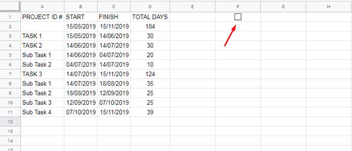
1. Sch – Master Data Sheet

This tab contains the actual schedule I want to share. I may update this often.

Note: There’s a tick box in cell F1 that we’ll use to control whether the data flows to the New tab. You can insert a tick box by going to Insert > Tick box.

Tick box in Sch tab used to control data flow to the New sheet in Google Sheets

2. New – Controlled Live Data

This tab conditionally pulls data from the Sch tab using this formula in A1:

=IF(Sch!F1=TRUE, ARRAYFORMULA(Sch!A1:D), "Please check back later")

If the tick box in Sch!F1 is checked, it pulls the data. If not, it displays a custom message.

3. Old – Manual Backup

Before editing the Sch tab, I manually copy-paste all values (except the tick box) into this Old tab as a backup.

4. Control – Choose What to Serve

This is the control panel where I decide whether the Destination File should receive data from the New tab or the Old tab.

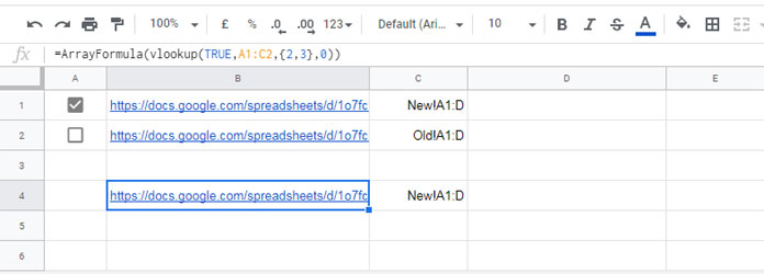
Control sheet setup to control reloading of IMPORTRANGE in Google Sheets using tick boxes and source tab URLs

Setting Up the Control Tab

In the Control tab:

Cells A1 and A2: Tick boxes
Cells B1 and B2: URLs of the New and Old tabs
Cells C1 and C2: Corresponding ranges to import

When tick box A1 is checked, we use the New tab. When A2 is checked, we use the Old tab.

Live demo of how tick box selection updates the formula to control reloading of IMPORTRANGE in Google Sheets

Here’s the formula in cell B4 of the Control tab:

=IF(
   COUNTIF(A1:A2, TRUE)=2, 
   "Only Select One Tick box at a time", 
   ARRAYFORMULA(IFNA(VLOOKUP(TRUE, A1:C2, {2,3}, 0)))
)

This outputs the selected URL and range for the next steps.

In the Source File:

Go to File > Share > Share with others, and set sharing to Restricted. Copy the file’s URL for later use.

The Mirror File (Bridge Sheet)

This is the middleman between the Source and Destination files — and a key part of how we control IMPORTRANGE reloading in Google Sheets.

Create a new Google Sheet named Mirror File. In cell A1 of a sheet named Mirror, enter:

=IMPORTRANGE(IMPORTRANGE("Source File URL", "'Control'!B4"), IMPORTRANGE("Source File URL", "'Control'!C4"))

Replace "Source File URL" with the actual URL of your source file.

Now, go to File > Share > Share with others, and change the sharing setting to:
Anyone with the link can view. Copy this link for use in the destination file.

The Destination File: Final Step

In the Destination File, enter the following formula in cell A1:

=IMPORTRANGE("Mirror File URL", "Mirror!A1:D")

Replace "Mirror File URL" with the actual link you copied.

How This Setup Controls IMPORTRANGE Reloading

Here’s how the setup works:

Source File Settings	What Destination File Sees
Tick box checked in `Sch!F1`	Live data is available
Control tab: A1 checked, A2 unchecked	Imports data from the `New` tab
Control tab: A2 checked, A1 unchecked	Imports data from the `Old` tab
Both tick boxes checked or both unchecked	Returns `#N/A!` (invalid condition)
Tick box unchecked in `Sch!F1` and `Control!A1` checked	Shows: “Please check back later”

This setup gives you manual control over reloading of IMPORTRANGE in the destination file — which is useful when you want to delay or schedule updates.

You can manually copy-paste data from the New tab to the Old tab as and when needed to maintain version control.

Wrapping Up: Control IMPORTRANGE Reloading in Google Sheets

This is how you can control reloading of IMPORTRANGE from the source file in Google Sheets. It’s not bulletproof, but it offers a practical workaround for giving you more control over when data updates flow through.

Give it a try and tweak it to fit your workflow!