Pull the Last Row from Multiple Sheets into One in Google Sheets

Want to pull just the last row from multiple sheets into one table in Google Sheets? Whether you’re consolidating monthly totals or summary rows into a dashboard, this guide will show you exactly how to do it, with formulas only, no Apps Script needed.

Table of Contents

Why Consolidate the Last Row from Multiple Sheets?

This method is helpful when:

Each sheet represents a month, and the last row contains monthly totals.
You want to create a dashboard that summarizes these totals in one place.
You don’t want to hardcode row numbers because rows may shift due to edits.

Hardcoding the last row number (e.g., Sheet1!A20:D20) can break easily. A formula-based approach is more robust.

Sample Data

Assume you have data in Sheet1 and Sheet2, each with four columns. The last row contains totals in columns 2 and 4.

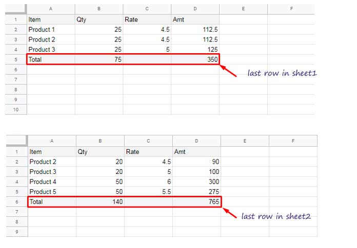
Our goal: Extract only the last row from each sheet and consolidate them.

Step 1: Extract the Last Row from Each Sheet

To get the last row with any data from Sheet1, use:

=CHOOSEROWS(Sheet1!A1:D, MAX(BYROW(Sheet1!A1:D, LAMBDA(val, IF(COUNTA(val), ROW(val))))))

This formula dynamically identifies the last row that contains any data across multiple columns.

To learn more about how this works, see:
Google Sheets: Get the Last Row with Any Data Across Multiple Columns

Repeat the same for Sheet2:

=CHOOSEROWS(Sheet2!A1:D, MAX(BYROW(Sheet2!A1:D, LAMBDA(val, IF(COUNTA(val), ROW(val))))))

Step 2: Stack the Last Rows Together

Now use VSTACK to combine the last rows from both sheets:

=VSTACK(
  CHOOSEROWS(Sheet1!A1:D, MAX(BYROW(Sheet1!A1:D, LAMBDA(val, IF(COUNTA(val), ROW(val)))))),
  CHOOSEROWS(Sheet2!A1:D, MAX(BYROW(Sheet2!A1:D, LAMBDA(val, IF(COUNTA(val), ROW(val))))))
)

This creates a new table with the last row from each sheet stacked vertically.

A	B	C	D
Total	75		350
Total	140		765

Step 3: Summarize the Consolidated Last Rows

Finally, use QUERY to group the data by the first column and summarize numeric columns:

=QUERY(
  VSTACK(
    CHOOSEROWS(Sheet1!A1:D, MAX(BYROW(Sheet1!A1:D, LAMBDA(val, IF(COUNTA(val), ROW(val)))))),
    CHOOSEROWS(Sheet2!A1:D, MAX(BYROW(Sheet2!A1:D, LAMBDA(val, IF(COUNTA(val), ROW(val))))))
  ),
  "SELECT Col1, SUM(Col2), SUM(Col4) GROUP BY Col1 LABEL SUM(Col2) '', SUM(Col4) ''"
)

This groups by Col1 (Item) and sums columns 2 and 4.

A	B	C
Total	215	1115

You can change the group or sum columns by editing the SELECT, GROUP BY, and LABEL parts.

Example:

To group by column 3 and sum column 2:

SELECT Col3, SUM(Col2) GROUP BY Col3 LABEL SUM(Col2) ''

Tip: The LABEL clause is used to rename or hide column headers in the output. If you change the columns in SELECT, you’ll likely want to update the corresponding LABEL entries as well to reflect new headers or leave them blank.