If you have chess pieces but lack a chessboard, don’t worry! You can easily create a chessboard in Google Sheets using conditional formatting and print it out. In this tutorial, I’ll provide you with a ready-to-use chessboard template in Google Sheets and the necessary formula to create one yourself.

A chessboard consists of 64 equal-sized squares, which you can create using an 8×8 grid in Google Sheets.

We will use conditional formatting to apply alternating colors—typically black and white—just like a real chessboard in Google Sheets.

While you could manually fill each cell, doing so for 64 squares can be tedious. Fortunately, there’s a simple formula that automates this task.

My goal in using conditional formatting instead of manual formatting is to introduce you to a custom formula in Google Sheets. This method also lets you generate a chessboard instantly.

If you want to play chess within Google Sheets, you can copy the chess pieces and paste them as values. This allows you to place and move the pieces on the board as needed.

Prerequisites

Before applying the custom formula in conditional formatting, ensure that the chessboard grid consists of square-shaped cells.

Resize Rows:

1. Select rows 1 to 10 by clicking row 1, holding Shift, and clicking row 10.
2. Right-click to open the context menu and choose “Resize rows 1-10.”
3. Enter 42 pixels as the row height (you can adjust this to fit within one screen).

Resize Columns:

1. Select columns A to J by clicking column A, holding Shift, and clicking column J.
2. Choose “Resize columns A-J”, enter 42 pixels, and click OK.

You can change the row and column sizes as needed, but make sure they have the same pixel dimensions.

Custom Conditional Format Rule to Apply a Chessboard Pattern

Now, let’s apply conditional formatting to fill the equally sized squares with alternating colors. The pattern should align diagonally, meaning a straight line from one corner of the board to the opposite corner should pass through squares of the same color.

Follow these steps to conditional format a chessboard in Google Sheets:

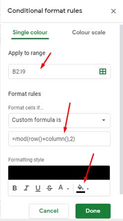
1. Select the 64 equal-sized cells by clicking B2, holding Shift, and clicking I9.
2. Go to Format > Conditional formatting.
3. Enter the following custom formula in the provided field:Formula:=MOD(ROW() + COLUMN(), 2)
4. Under formatting style, select black as the fill color.
5. Click Done.

Your chessboard in Google Sheets is now ready!

To better visualize the setup, please refer to the image below.

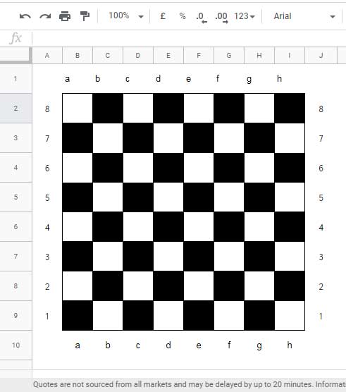
In this chessboard, I have also included algebraic notation, which can help describe chess moves. Additionally, I removed the gridlines via the View menu.

How to Get Symbols for Black and White Chess Pieces in Google Sheets

If you want to play chess within Google Sheets, in addition to formatting the chessboard pattern, you will need the chess pieces.

Using the CHAR function, you can insert the symbols of chess pieces and pawns in Google Sheets. Below are the corresponding formulas:

Black Pieces

White Pieces

Playing Chess Within Google Sheets

Now that we have formatted the chessboard and have the necessary pieces, you can play a game within Google Sheets.

To do this:

1. Replace the black color in the grid with dark orange 1 or another distinguishable shade.
2. Select the grid and apply the following formatting:
   • Font Size: 20
   • Vertical Align: Center
   • Horizontal Align: Center
3. Copy the chess piece symbols and paste them as values (right-click > Paste special > Values only).

This setup allows you to play chess with a friend directly in Google Sheets!

Chessboard Download

Resources

• Inserting Bullet Points in Google Sheets
• Rate with Ease: Google Sheets’ New Built-In Rating Feature
• 5-Star Rating in Google Sheets Including Half Stars
• Inserting Bullet Points in Google Sheets
• Insert Special Characters Without an Add-on in Google Sheets
• Smileys and Icons Based on Values in Google Sheets