Compare Two Rows and Find Matches in Google Sheets

Need to verify if two rows in your Google Sheet contain the same values? Whether you’re double-checking data entry, comparing quiz answers, or validating records, this guide shows you how to compare two rows in Google Sheets—either column by column or by checking for matches across rows regardless of position.

Table of Contents

Option 1: Compare Two Rows Column by Column and Find Exact Matches

If you want to compare two rows side by side—cell by cell—Google Sheets makes it easy with simple logical formulas.

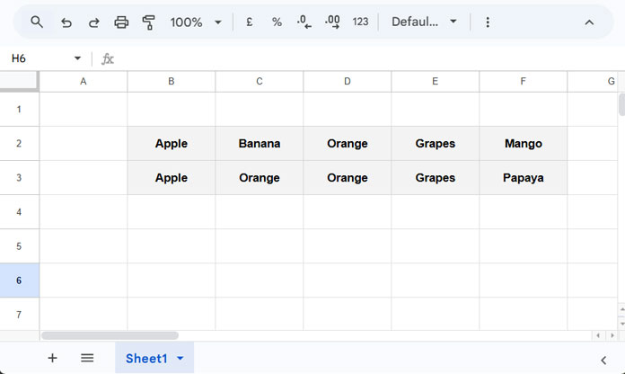
Let’s say you want to compare the values in the range B2:F2 with the values in B3:F3.

Sample data showing two rows of fruit names (B2:F2 and B3:F3) to compare column by column in Google Sheets

Formula to Compare Row Values by Column

You can use this formula in cell B4 and drag it across:

=B2=B3

This will return TRUE where the values match and FALSE where they don’t.

Array Formula to Compare Entire Rows

To avoid dragging the formula across, use this array version in B4:

=ArrayFormula(B2:F2 = B3:F3)

This will output a row of Boolean values comparing each column in Row 2 with the corresponding column in Row 3.

When to Use Each

Drag-across formula – Ideal for conditional formatting
ArrayFormula – Useful for filtering or summarizing comparison results

Example: Highlight Mismatching Values with Conditional Formatting

To highlight cells where values don’t match between Row 2 and Row 3:

Select the range B2:F3
Go to Format > Conditional formatting
Under Format rules, choose Custom formula is
Enter this formula:
=NOT(B$2 = B$3)

Apply a fill color of your choice, and mismatched cells will be highlighted.

Highlighted mismatched cells between two rows in Google Sheets using conditional formatting to compare values column by column

Example: Filter Only Mismatching Columns

To extract only the columns where values don’t match:

=FILTER(B2:F3, NOT(B2:F2 = B3:F3))

This returns a subset of both rows showing only the differing values:

Banana	Mango
Orange	Papaya

Real-Life Use Cases for Column-by-Column Comparison

Compare quiz responses from two attempts
Validate form submissions or data entry
Check for differences in product attributes
Audit manual vs automated entries

Option 2: Find Values That Match Anywhere Across Rows

In some scenarios, you may want to compare two rows without caring about column positions—just whether the values exist anywhere in the other row.

This is especially helpful when you’re dealing with unordered lists like tags, ingredients, or multi-select responses.

Filter Values in Row 2 That Exist in Row 3

=FILTER(B2:F2, XMATCH(B2:F2, B3:F3))

Filter Values in Row 2 That Don’t Exist in Row 3

=FILTER(B2:F2, ISNA(XMATCH(B2:F2, B3:F3)))

Reverse the Comparison (Row 3 in Row 2)

To check whether values in Row 3 exist in Row 2:

=FILTER(B3:F3, XMATCH(B3:F3, B2:F2))

To find non-matching values:

=FILTER(B3:F3, ISNA(XMATCH(B3:F3, B2:F2)))

Tip: Remove Duplicates from Filtered Results

If your filtered result contains duplicates, you can wrap it with UNIQUE like this:

=UNIQUE(FILTER(...), TRUE)

Just replace FILTER(...) with the relevant filter formula.

Wrapping Up

That’s how you can compare two rows and find matching or mismatching values in Google Sheets—either column by column or across the entire row. Both methods are useful depending on whether position matters in your comparison.