To compare two sets of multi-column data (two tables) for differences in Google Sheets, there must be a unique column in both tables.

For example, in an employee database, this could be the Employee ID or Employee Name. In a product database, it might be the Product Code or Product Name.

We’ll use an advanced technique involving a helper formula and conditional formatting to achieve this task. This method highlights cells in either table that differ from the corresponding cells in the other table.

What makes my approach exciting is that the records don’t need to be in the same order; the unique IDs in the two tables don’t have to match row by row.

We’ll utilize an advanced XLOOKUP formula to identify mismatched values in each record and use the formula’s output to highlight the relevant cells.

Let’s consider two employee databases as examples. We will compare these two multi-column datasets and identify differences, such as changes in salary, addition of new employees, and more.

Sample Data

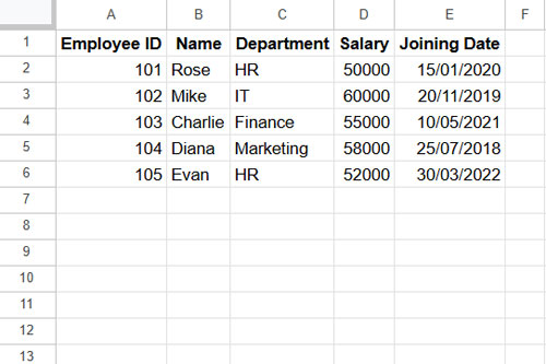
Below is the sample data in Sheet1 with fields: Employee ID, Name, Department, Salary, and Joining Date:

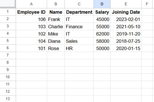
And here is the sample data in Sheet2 with the same field labels:

We will use Employee ID as the unique identifier to compare these two sets of multi-column data for differences.

Step 1: Choosing the Table to Highlight

There are two tables, and you can choose which one you want to compare and highlight for differences. You can highlight differences in either or both tables.

Let’s start by highlighting the multi-column data in Sheet1 for differences.

Step 2: Formula to Compare Two Sets of Multi-Column Data

Navigate to cell G2 of Sheet1 and enter the following formula:

=ArrayFormula(IFNA(BYCOL(Sheet2!A2:E, LAMBDA(col, XLOOKUP(A2:A, Sheet2!A2:A, col)))=A2:E))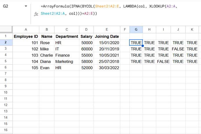

Explanation of the Formula:

• A2:E: The range of the table in Sheet1.
• Sheet2!A2:E: The range of the table in Sheet2.
• A2:A: The unique ID column in Sheet1.
• Sheet2!A2:A: The unique ID column in Sheet2.

This formula returns an array with TRUE or FALSE values:

• FALSE indicates the value is different in the second table.
• Empty rows indicate that the record is not present in the second table.

We’ll now use this array to highlight the differences.

Step 3: Highlighting Differences

1. Select A2:E in Sheet1.
2. Go to Format > Conditional Formatting.
3. Under Format Rules, select Custom Formula is.
4. Enter the following formula: =AND(LEN(A2), NOT(G2))
5. Choose a fill color for highlighting.
6. Click Done.

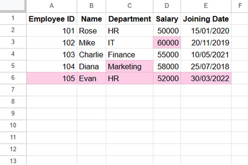
This will highlight the values in Sheet1 that don’t match the corresponding values in Sheet2.

Compare and Highlight Differences in Both Tables

If you want to compare the data in Sheet2 with Sheet1 and highlight the differences:

1. Enter the same formula in Sheet2!G2, modifying the range references:
   • Replace Sheet2!A2:E with Sheet1!A2:E.
   • Replace Sheet2!A2:A with Sheet1!A2:A.
2. Apply the same conditional formatting rule in Sheet2 to highlight the differences.

Formula Breakdown

Here’s a detailed breakdown for those interested in learning the formula:

=ArrayFormula(IFNA(BYCOL(Sheet2!A2:E, LAMBDA(col, XLOOKUP(A2:A, Sheet2!A2:A, col)))=A2:E))

1. XLOOKUP(A2:A, Sheet2!A2:A, Sheet2!A2:A): Looks up the Employee IDs in A2:A of Sheet1 within Sheet2!A2:A and returns the matching rows. (To test it, enter it as an array formula by wrapping it with the ARRAYFORMULA function.)
2. Custom Function: To fetch values from all columns in Sheet2, use a LAMBDA function (by modifying the above XLOOKUP formula): LAMBDA(col, XLOOKUP(A2:A, Sheet2!A2:A, col))
3. BYCOL(Sheet2!A2:E, ...): BYCOL applies the LAMBDA function to each column in Sheet2!A2:E.
4. IFNA: Replaces #N/A errors (from mismatched rows) with blank values.
5. =A2:E: Compares the fetched values from Sheet2 with the values in Sheet1. Returns TRUE for matches and FALSE for mismatches.

Additional Resources

Here are some more Google Sheets resources related to comparing values:

• Compare Two Sheets in Google Sheets and Identify Differences
• How to Compare Two Columns for Matching Values in Google Sheets
• Compare Two Tables and Remove Duplicates in Google Sheets
• Google Sheets: Compare Two Lists and Extract Differences
• Compare Two Google Sheets Cell by Cell and Highlight
• Compare Two Rows and Find Matches in Google Sheets
• Compare All Columns with Each Other for Duplicates in Google Sheets