You can use the INDEX, OFFSET, or CHOOSECOLS function in combination with the ROW function to change column letters when a formula is copied or dragged down in Google Sheets.

In other words, when dragging down the fill handle of a formula cell, the row position should remain absolute, while the column position changes dynamically.

Change Column Letter When Copying Formulas Down: Explained

For example, the formula =A1 should change to =B1, =C1, =D1, and so on, when copied down, instead of changing the row numbers to =A2, =A3, =A4, and so on.

In essence, this method ensures that column letters change when a formula is copied down in a single column.

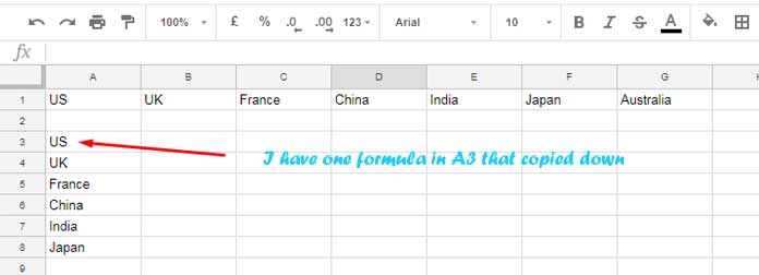
Let’s look at the following example:

You have country names in row 1 spanning the range A1:G1.

In cell A3, you want to write a formula that starts with =A1. When you copy this formula down to A4, A5, A6, and so on, the resulting values should come from B1, C1, D1, etc., instead of moving to A2, A3, A4.

Typically, when formulas are copied down, the column reference remains static, and only the row reference changes. For instance:

• The formula in cell A3 is =A1.
• When copied to A4, it becomes =A2.

But in this case, we want:

• =A1 in A3,
• =B1 in A4,
• =C1 in A5, and so on.

Now, let’s explore formulas that allow column letters to change when a formula is copied down.

Formulas to Change Column Letters When Copying Down

1. Using OFFSET and ROW

=OFFSET($A$1, 0, ROW(A1)-1)

• Explanation:
  The OFFSET function has the syntax OFFSET(reference, offset_rows, offset_columns).
  • reference: The starting cell, $A$1.
  • offset_rows: Set to 0 since we don’t want to offset rows.
  • offset_columns: Uses ROW(A1)-1, which dynamically adjusts the column offset based on the row number.
• How It Works:
  Initially, ROW(A1)-1 evaluates to 0, so the formula points to A1.
  When copied down, ROW(A2)-1 becomes 1, offsetting the column by one, resulting in B1.
• Example Usage:
  Replace $A$1 with $E$10 if you want values from E10, F10, G10, and so on, when copying the formula down.

2. Using INDEX and ROW

=INDEX($A$1:$Z$1, 1, ROW(A1))

• Explanation:
  The INDEX function has the syntax INDEX(reference, [row], [column]).
  • reference: The row range, $A$1:$Z$1.
  • row: Set to 1, indicating the first row in the range.
  • column: Uses ROW(A1), dynamically adjusting the column index.
• How It Works:
  Initially, ROW(A1) returns 1, so the formula fetches the value from column 1 (A1).
  When copied down, ROW(A2) becomes 2, fetching the value from column 2 (B1).

3. Using CHOOSECOLS and ROW

=CHOOSECOLS($A$1:$Z$1, ROW(A1))

• Explanation:
  The CHOOSECOLS function returns values from specific columns in the provided range.
  • The range is $A$1:$Z$1.
  • The column index is determined by ROW(A1).
• How It Works:
  Initially, ROW(A1) returns 1, fetching the value from column 1 (A1).
  When copied down, ROW(A2) becomes 2, fetching the value from column 2 (B1), and so on.
• Why Use CHOOSECOLS?
  It’s a simpler, more modern approach for this task and avoids manual offsets or complex references.

Summary

Each of these formulas provides a way to dynamically adjust column letters while dragging a formula down. Depending on your preference and use case, you can use OFFSET, INDEX, or CHOOSECOLS.

This approach is particularly useful for scenarios where you want row data to populate a column dynamically as the formula is dragged down.

Resources

• Move Values from Alternate Rows to Columns in Google Sheets
• How to Move Each Set of Rows to Columns in Google Sheets
• Drag Formula Right, Increment Cell Reference Down in Google Sheets