
 in Google Sheets")

")


")


")


How to properly use a cell reference in the filter menu, filter by condition, custom formula field in Google Sheets?
I am going to just include one example to make you understand the proper use of cell reference in the Filter menu in Google Sheets. That example included in the last part of this guide.
This technique/tip I’ll use in one or a few of my upcoming tutorials related to advanced filtering using the Filter menu command.
Let’s start with an introduction to the Filter menu in Google Sheets.
Introduction
Google Sheets has one dedicated function to help you organize and analyze your data. It’s none other than the FILTER function.
There is one more function named QUERY, which has the same capability. But I don’t call it a dedicated FILTER function as it’s more versatile.
Still many are using the Filter menu command over the said two functions. Why?
The reason to use the Filter menu over the said functions is simple. The formulas based on the functions create a new filtered range, which many users don’t want. Other than this, there is one more advantage.
I’m sure you are aware of the two types of Filter menu commands – ‘Create a Filter’ and ‘Filter View’ (for creating a filtered view, both you can access from the Data menu).
The ‘Filter Views’ are only viewable/accessible on a computer. This has one benefit. Different users can set different filters on a data set. Needless to say, it’s no way possible with a single formula.
Proper Use of Cell Reference in Filter Menu Custom Formula Field
Let’s come to the point, i.e. using cell reference in formulas in the filter menu in Google Sheets.
You can use formulas in Google Sheets;
- Within a cell/range.
- As a custom formula in the following menu command fields.
- Data Validation.
- Conditional formatting.
- Filter menu.
We all use cell references in formulas for referring to a cell or an array/range. But the usage is slightly different when it comes to formulas within a cell and formulas within menu commands.
I am leaving the Data Validation and Conditional Formatting this time. Let’s focus on the Filter menu and how to properly use a cell reference in it. See the example below.
Note: As the name denotes, the purpose of the Filter menu, ‘Filter by condition’ is to use a custom formula to filter the corresponding column.
How to Insert a Custom Formula in the Filter Menu in Google Sheets
Sample Data:
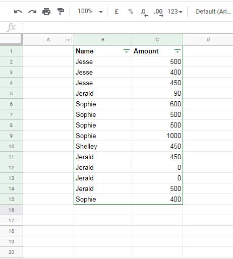
I have already set a filter to the range B1:C15. To do that follow the below steps.
- Select the range B1:C15.
- Then go the menu Data and click on ‘Create a filter’.
To insert a custom formula, just follow the below 3 steps.
- Assume you want to filter a name in column B. So click on the drop-down in cell B1.
- Then click on the ‘Filter by condition’
- Finally, select ‘Custom formula is’.
Cell Reference in Formulas in Filter Menu Filter by Condition in Google Sheets
We may use a cell reference in a Filter menu formula either to refer to the data in a column or a cell contains a condition/criterion.
Cell Reference to Data in a Column
Now I just want to filter the name ‘Jesse’ using a custom formula. How to do this?
=B2="Jesse"Just insert the above formula in the blank field just below the ‘Custom formula is’ field and click “OK”.
No need to refer to the entire range B2:B15 in the formula as =B2:B15="Jesse" or =ArrayFormula(B2:B15="Jesse")
The above is tip # 1 to the proper use of cell reference in Filter menu in Google Sheets. See tip # 2 below.
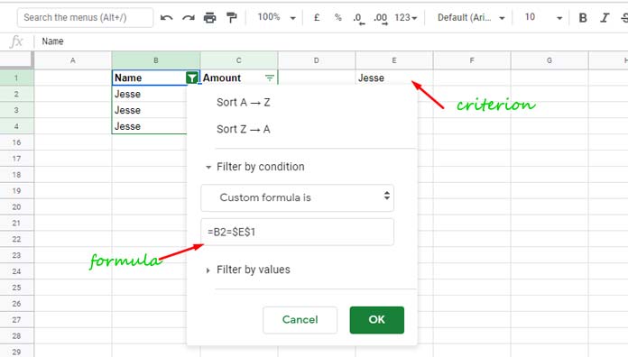
Cell Reference to Criterion in a Cell
The above Filter menu formula has one problem. Whenever you want to filter the data with a new condition you need to edit the formula to change the condition/criterion.
So the ideal way is to insert the criterion, here the name “Jesse”, in a cell and in the formula, make a reference to that cell. So that you can later change the name “Jesse” with some other criterion.
Assume I have entered the name “Jesse” in cell E1. Then the proper way to use the cell references to this cell in the Filter menu ‘Filter by condition’ custom formula in Google Sheets is as follows.
=B2=$E$1You must use an absolute cell reference to refer to the criterion cell (see the dollar sign). Regarding the cell referring to the data (B2), it must be kept as relative (no dollar sign).
If you make any mistake in using the cell reference as said above, you will see blank data or improper filtering.
Please note that changing the criterion in cell E1 itself won’t prompt the filter menu to apply a new filter accordingly! Then?
Once you have changed the criterion, click on the drop-down in cell B1 and simply click “OK”.
Hello,
Can I use a custom formula that has a ‘contains text…’ and reference another cell in the sheet.
Hi, joanna ward,
Please share an example.
Useful information. Thank you.