This tutorial provides a solution for incorporating case sensitivity into the running count of values in Google Sheets.
This is particularly useful when dealing with case-sensitive codes or terms such as product codes, customer names, IDs, and more.
A running count tracks the number of occurrences of values in a column. If a value repeats three times, the formula numbers it 1, 2, 3, regardless of its position in the column. Multiple values will also be numbered in the same pattern.
A case-sensitive running count is an advanced version of this, where values are differentiated based on their case. For example, the formula treats “Apple” and “APPLE” as two distinct values.
Non-Array Formula
We’ll start with a non-array formula. Assume the values are in A2:A.
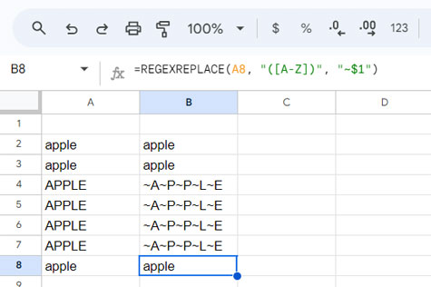
Enter the following REGEXREPLACE formula in cell B2, which prefixes each capital letter in cell A2 with “~”:
=REGEXREPLACE(A2, "([A-Z])", "~$1")Drag this formula down as far as needed.

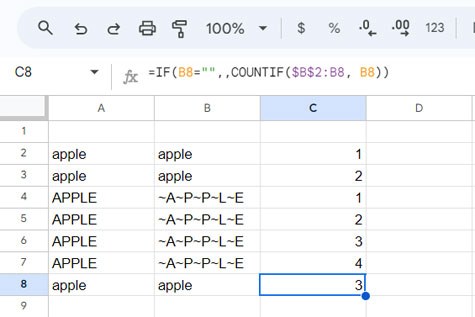
In cell C2, enter the following COUNTIF formula:
=IF(B2="",,COUNTIF($B$2:B2, B2))Drag this formula down as far as needed.

The COUNTIF formula counts the occurrences of the current value within the range up to the current row. As you drag the formula down, B2 (the current value) becomes B3, B4, and so on, while the range $B$2:B2 expands to $B$2:B3, $B$2:B4, and so forth.
This is the non-array solution for getting a case-sensitive running count in Google Sheets.
Array Formula for Case-Sensitive Running Count
If you prefer to avoid dragging formulas and using helper ranges, you can use this array formula.
Generic Formula for Case-Sensitive Running Count:
=ArrayFormula(
   IF(
      range="",,
      COUNTIFS(
         REGEXREPLACE(range, "([A-Z])", "~$1"),
         REGEXREPLACE(range, "([A-Z])", "~$1"),
         ROW(range),
         "<="&ROW(range)
      )
   )
)
Here, range refers to the range of values for which you want to get the case-sensitive running count of occurrences.
Example:
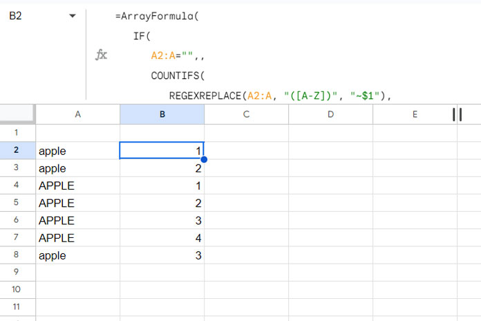
In the following example, the range is A2:A and the following formula is in cell B2:
=ArrayFormula(
   IF(
      A2:A="",,
      COUNTIFS(
         REGEXREPLACE(A2:A, "([A-Z])", "~$1"),
         REGEXREPLACE(A2:A, "([A-Z])", "~$1"),
         ROW(A2:A),
         "<="&ROW(A2:A)
      )
   )
)
Since this is an array formula, ensure that the range B2:B is empty before applying the formula to avoid a #REF! error.

Formula Explanation
The array formula is essentially a COUNTIFS formula, which follows this syntax:
COUNTIFS(
   criteria_range1,
   criterion1,
   [criteria_range2, …],
   [criterion2, …]
)
In our case-sensitive running count formula, the arguments are as follows:
- criteria_range1:
REGEXREPLACE(A2:A, "([A-Z])", "~$1") - criterion1:
REGEXREPLACE(A2:A, "([A-Z])", "~$1") - criteria_range2:
ROW(A2:A) - criterion2:
"<=" & ROW(A2:A)
If you use only criteria_range1 and criterion1, the COUNTIFS will count the occurrences of each value in the entire range.
E.g.:
| apple | 3 |
| apple | 3 |
| APPLE | 4 |
| APPLE | 4 |
| APPLE | 4 |
| APPLE | 4 |
| apple | 3 |
To limit the count to a growing range, criteria_range2 and criterion2 are used. These ensure that the COUNTIFS formula evaluates whether the row number of the range is less than or equal to the row number of the current row. This approach restricts the count to the portion of the range up to the current row.
The IF logical test returns empty values ("") in rows where the cell value is empty in the range. The ARRAYFORMULA ensures that the non-array function is applied across the entire range.
Tip: Boosting Case-Sensitive Running Count Performance
To enhance the performance of the case-sensitive running count array formula, use the LET function to avoid repeating calculations.
Here’s the optimized formula:
=ArrayFormula(
   LET(
      range, A2:A,
      regex, REGEXREPLACE(range, "([A-Z])", "~$1"),
      row_n, ROW(range),
      IF(
         range="",,
         COUNTIFS(regex, regex, row_n, "<="&row_n)
      )
   )
)
For related tutorials, please check out the resources provided.


