


")


")

")
")
 in Excel & Google Sheets")


Case-sensitive Reverse VLOOKUP refers to looking up a search key in a column case-sensitively and returning the corresponding value from a column to the left. How can we do this in the example below? Is it a complex task?
| Date | Item Code | Qty |
| 21/09/2024 | PRT 500 AA | 100 |
| 22/09/2024 | PRT 500 Aa | 75 |
| 23/09/2024 | HRD 129 Y | 100 |
| 24/09/2024 | PRT 900 X | 150 |
| 25/09/2024 | HRD 129 y | 90 |
We can achieve this using VLOOKUP with EXACT or INDEX-MATCH with EXACT. In terms of complexity, it’s a relatively simple task.
In the following example, we will case-sensitively look up an item code in column B and return the corresponding date from column A. This can be called a case-sensitive reverse (leftward) lookup in Google Sheets.
In this example, PRT 500 AA and PRT 500 Aa are distinct, showing the case sensitivity of the lookup.
Example of Case-Sensitive Reverse VLOOKUP
The following formula in cell F2 will look up PRT 500 Aa entered in cell E2 in column B and return the date 22/09/2024 from column A.
=ArrayFormula(
   VLOOKUP(TRUE, HSTACK(EXACT(B2:B6, E2), A2:A6), 2, FALSE
   )
)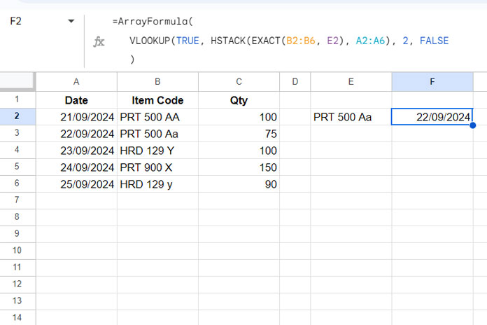
Unlike in Excel, you can extend the ranges B2:B6 and A2:A6 to B2:B and A2:A, allowing the formula to include future values in these columns.
Let me explain this formula step-by-step. Then we will move on to case-sensitive reverse VLOOKUP using an alternative INDEX-MATCH method.
Formula Breakdown
Syntax: VLOOKUP(search_key, range, index, [is_sorted])
Since VLOOKUP function can only search the first column of a range, for case-sensitive reverse VLOOKUP, we need to adjust the range accordingly.
- Range:
HSTACK(EXACT(B2:B6, E2), A2:A6)where: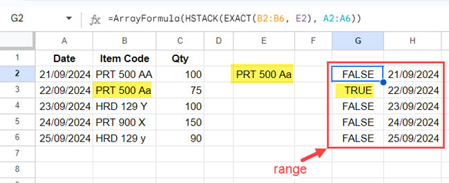
EXACT(B2:B6, E2)checks if the text in E2 exactly matches each text in B2:B6, returning an array of TRUE or FALSE, with TRUE representing an exact match. This function needs ARRAYFORMULA to handle comparisons across a range.- HSTACK horizontally stacks the A2:A6 range alongside the array of TRUE/FALSE values, creating a two-column array for the lookup.
VLOOKUP(TRUE, …)searches for the first TRUE in the new virtual range and returns the corresponding value from the second column (the date).- The last argument FALSE ensures we are doing an exact match rather than a partial match, as the range is not sorted.
INDEX-MATCH Alternative for Case-Sensitive Reverse VLOOKUP
This is an alternative to the above VLOOKUP formula:
=INDEX(A2:A6, MATCH(TRUE, EXACT(B2:B6, E2), 0))This method is quite straightforward if you’ve reviewed the case-sensitive VLOOKUP example above.
EXACT(B2:B6, E2)returns an array of TRUE or FALSE, where TRUE represents an exact match.- The MATCH function finds the first occurrence of TRUE in this array and returns the relative position.
- The INDEX function uses that position to retrieve the corresponding value from the date column.
Since INDEX operates as an array formula, the use of the ARRAYFORMULA function is not necessary for EXACT.
It’s that simple! Test both formulas and see which one you prefer. I recommend using INDEX-MATCH for case-sensitive reverse VLOOKUP due to its simplicity.