


")


")

")
")
 in Excel & Google Sheets")


Let me start with a question: Do you know when to use the AVERAGEA function in Google Sheets?
If you’re unsure, it’s likely because you don’t yet know the purpose of the AVERAGEA function.
The AVERAGEA function calculates the average (arithmetic mean) of a set of values, including numbers, text, and Boolean values (TRUE, FALSE), in a range or list of arguments.
There are several other functions for calculating averages:
We’ll explore how the AVERAGEA function differs from these alternatives after we review its syntax and arguments.
AVERAGEA Function Syntax, Arguments, and Examples in Google Sheets
Syntax:
AVERAGEA(value1, [value2, ...])Arguments:
value1– The first value or range to include in the average.- Example (single value):
=AVERAGEA(100) - Example (range):
=AVERAGEA(A1:A10)
- Example (single value):
value2– (Optional) Additional values or ranges to include.- Example (multiple values):
=AVERAGEA(100, 150) - Example (multiple ranges):
=AVERAGEA(A1:A10, C1:C10)
- Example (multiple values):
Google Sheets supports an arbitrary number of arguments in an AVERAGEA formula, even though documentation may suggest a limit of 30.
Note: value1 is required; value2, value3, and so on are optional.
Difference Between AVERAGE and AVERAGEA in Google Sheets
Here’s a quick comparison to help you understand how AVERAGE and AVERAGEA treat different types of data:
| Range Contains | AVERAGE | AVERAGEA |
|---|---|---|
| Text | Ignores | Converts to 0 and includes |
| Blank (empty cell) | Ignores | Ignores |
| Number | Includes | Includes |
| TRUE | Ignores | Converts to 1 and includes |
| FALSE | Ignores | Converts to 0 and includes |
| Error | Returns error | Returns error |
When to Use AVERAGEA
Let’s look at an example where only AVERAGEA can give the correct result, while other functions may return #DIV/0!.
Say you want to calculate the average number of students who scored greater than or equal to 80 in an exam. You have the marks of 20 students in column D.
First, enter the following formula in cell E2 to check which students meet the criteria:
=ArrayFormula(D2:D21 >= 80)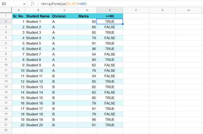
Note: This formula covers rows 2 to 21. Ensure cells E2:E21 are empty before using it.
This returns TRUE for scores ≥ 80 and FALSE otherwise.
Now use the AVERAGEA function to calculate the mean:
=AVERAGEA(E2:E21)The function will treat TRUE as 1 and FALSE as 0, giving you the proportion of students who scored at least 80.
Use AVERAGEA Without Helper Column
You can simplify the formula using just one cell:
=ArrayFormula(AVERAGEA(D2:D21 >= 80))Alternatively, if you prefer to use the standard AVERAGE function, you can convert the Boolean values to numbers like this:
=ArrayFormula(AVERAGE(--(D2:D21 >= 80)))Conditional Average: DAVERAGE, AVERAGEIF, and AVERAGEIFS
We often compare the AVERAGE and AVERAGEA functions. However, when applying conditions, other functions such as DAVERAGE, AVERAGEIF, and AVERAGEIFS become more suitable.
These functions can filter data based on conditions and then compute the average.
Without conditions, they behave similarly to AVERAGE—they ignore text, TRUE, and FALSE values.
To apply conditions with AVERAGE or AVERAGEA, you need to wrap them in a FILTER or use a QUERY.
Let’s find the average marks of students in Division B using different functions (assuming relevant sample data exists in columns C and D):
AVERAGEIF
=AVERAGEIF(C2:C21, "B", D2:D21)AVERAGEIFS
=AVERAGEIFS(D2:D21, C2:C21, "B")DAVERAGE
=DAVERAGE(A1:E21, 4, {"Division"; "B"})Bonus Tip: Check out Mastering Criteria in Database Functions in Google Sheets for a deeper dive.
AVERAGE with FILTER
=AVERAGE(FILTER(D2:D21, C2:C21 = "B"))AVERAGEA with FILTER
=AVERAGEA(FILTER(D2:D21, C2:C21 = "B"))That’s everything you need to know about using the AVERAGEA function in Google Sheets! Thanks for reading — I hope it helped!