I want to calculate the average of values only in the visible rows in Google Sheets. How can I do that? Specifically, how can I exclude the hidden rows?
In this tutorial, you’ll learn how to calculate the average of visible rows in Google Sheets, excluding filtered, grouped, or manually hidden rows.
There are three common average functions in Google Sheets: AVERAGE, AVERAGEIF, and AVERAGEIFS. However, none of them support excluding hidden rows directly, so you need some workarounds.
Additionally, the QUERY function can also be used to calculate averages in Google Sheets, but again, workarounds are necessary to exclude hidden rows from the calculation.
You’ll learn those workarounds in this Google Sheets tutorial.
In this tutorial, I’ll give you several examples using the functions mentioned above with filtered data. I’m also expanding this tutorial to include how to handle rows hidden via row grouping in Google Sheets.
With that said, let’s dive in! Here’s what you will learn in this tutorial:
- How to calculate the average in Google Sheets while excluding filtered rows, hidden rows (via row grouping), and manually hidden rows.
- How to calculate a single conditional average, excluding the rows mentioned above.
- How to calculate multiple conditional averages, excluding filtered, grouped, and manually hidden rows.
- How to use the QUERY function to calculate averages in Google Sheets, excluding filtered, hidden, and grouped rows.
Average of Visible Rows
Average Excluding Filtered or Hidden Rows (Unconditional Average)
What is an average, and how do you calculate it? Before jumping into the examples, let’s cover this basic concept.
Average = Total / Count
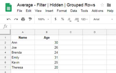
Let’s say you have the following data in columns A and B:
To calculate the total:
=B2 + B3 + B4 + B5 + B6 + B7or more efficiently:
=SUM(B2:B7)The total is 156.
To calculate the count:
=COUNT(B2:B7)The count is 6.
Now, to calculate the average:
=SUM(B2:B7) / COUNT(B2:B7)Alternatively, you can use the AVERAGE function:
=AVERAGE(B2:B7)The result would be 26.
Now, let’s introduce a filter. Suppose you want to filter out gender “M” (Male) and calculate the average of the remaining data. Follow these steps:
Select the range A1:C7 and apply Data > Create a filter.
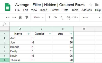
Click the filter icon in cell B1 (Gender column) and uncheck “M.”
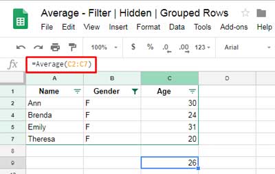
Now, if you try to calculate the average using the formula =AVERAGE(C2:C7), the result will be incorrect because it still includes the hidden rows.
The correct answer should be:
=(30 + 24 + 31 + 20) / 4 = 26.25To exclude filtered-out rows from the average calculation, we need to use an alternative approach with the SUBTOTAL function.
Average of Visible Rows in Google Sheets Using the SUBTOTAL Function
Using Function 1 to Exclude Filtered Rows
The SUBTOTAL function can be used to calculate averages while excluding filtered rows. Use function number 1 for this purpose:
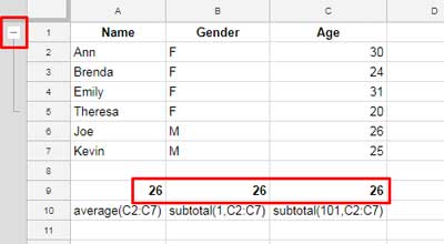
=SUBTOTAL(1, C2:C7)This formula calculates the average for visible rows, excluding any filtered rows. However, it includes manually hidden rows and rows hidden by row grouping.
Using Function 101 to Exclude Filtered, Hidden, and Grouped Rows
To exclude all hidden rows, including manually hidden rows and grouped rows, use function number 101:
=SUBTOTAL(101, C2:C7)This formula only considers visible rows for the average calculation.
Difference Between Function 1 and 101 in Google Sheets
SUBTOTAL(1, ...)calculates the average of visible rows, excluding filtered rows but including manually hidden rows and rows hidden by grouping.SUBTOTAL(101, ...)excludes filtered, manually hidden, and grouped rows.
Here’s an example: If rows 2, 3, and 4 are hidden by grouping, the result from SUBTOTAL(1, ...) will still include those rows, but SUBTOTAL(101, ...) will not.
Conditional Averages Excluding Hidden Rows
Single Conditional Average Excluding Filtered or Hidden Rows
Let’s say you want to calculate the average age for females (gender = “F”) in the list, while excluding hidden rows.
You can use the AVERAGEIF function:
=AVERAGEIF(B2:B7, "F", C2:C7)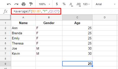
This formula will give you the average of all females’ ages, but it will not exclude hidden rows (whether filtered, grouped, or manually hidden). There is no SUBTOTALIF function in Google Sheets.
Workaround Using a Helper Column for Conditional Averages
To exclude hidden rows in a conditional average calculation, we can use a helper column with the SUBTOTAL function.
In column D (the helper column), enter the following formula in D2 and drag it down through D7:
=SUBTOTAL(109, C2)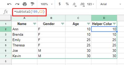
The function number 109 here is used for summing visible values (excluding hidden rows), similar to how 101 works for averages.
Now, you can use AVERAGEIFS to calculate the conditional average while excluding hidden rows:
=AVERAGEIFS(C2:C7, B2:B7, "F", D2:D7, ">0")This formula will only calculate the average for visible rows where the gender is “F” and the value in the helper column is greater than 0 (indicating the row is visible).
Alternatively, you can replace the helper column with a MAP formula:
=AVERAGEIFS(C2:C7, B2:B7, "F", MAP(C2:C7, LAMBDA(r, SUBTOTAL(109, r))), ">0")Multiple Conditional Averages Excluding Filtered or Hidden Rows
You can also calculate multiple conditional averages, excluding filtered, grouped, and hidden rows, by adding more conditions to the AVERAGEIFS function.
For example:
=AVERAGEIFS(C2:C7, B2:B7, "F", D2:D7, ">0", C2:C7, ">20")This formula will average the ages of females (gender = “F”), considering only visible rows where the age is greater than 20.
Using the QUERY Function to Calculate the Average of Visible Rows
You can replace the AVERAGEIFS formula with a QUERY formula to excludes hidden rows. Use the following formula:
=QUERY({A2:D7}, "SELECT AVG(Col3) WHERE Col2 = 'F' AND Col4 > 0 LABEL AVG(Col3)''")This formula uses the helper column to exclude hidden rows from the average calculation.
Or, if you want to eliminate the helper column, you can use a MAP function inside the query:
=QUERY({A2:C7, MAP(C2:C7, LAMBDA(r, SUBTOTAL(109, r)))}, "SELECT AVG(Col3) WHERE Col2 = 'F' AND Col4 > 0 LABEL AVG(Col3)'' ")Note: The QUERY function is case-sensitive, so ensure the case in your conditions matches your dataset.
Conclusion
In this tutorial, we explored how to calculate the average of visible rows in Google Sheets, excluding filtered, hidden, and grouped rows. The SUBTOTAL function plays a key role in handling hidden rows, and AVERAGEIFS combined with a helper column offers an effective solution for conditional averages.
From now on, you’ll be able to calculate averages accurately, even with hidden or filtered data in your Google Sheets!
Related:


