Sometimes you need to auto-populate a row from above in Google Sheets when a value repeats—like filling in product details automatically when you enter the same product code again. This saves time and prevents errors by reducing manual data entry. In this post, I’ll show you how to do this easily with the XLOOKUP function.
Let’s look at a common use case to understand how this works.
Example Scenario: Repeating Product Codes
Say you’re building a purchase log. You enter:
- Item Code in column A
- Item Name in column B
- Price per Ton in column C
- and maybe more fields like quantity, purchase date, etc.
Here’s the setup:
| A | B | C |
|---|---|---|
| Item Code | Item Name | Price / Ton |
| C-001 | Road Base | 3.5 |
This first record is manually entered. Now, let’s say later in the sheet you enter the same item code again — like in row 6. You want the sheet to automatically fill in the item name and price based on the previous entry.

That’s exactly where XLOOKUP helps.
How Is This Different from Google Sheets’ Autocomplete?
Google Sheets has a built-in autocomplete feature that suggests values based on what you’ve typed in previous cells. While helpful, autocomplete is just a visual prompt — it doesn’t actually fill in data or update other cells automatically.
In contrast, the XLOOKUP method we’re using here auto-populates cells based on values already entered above — the data is pulled by formula and saved in the cell. It’s dynamic and updates automatically if previous entries change.
How to Auto-Populate a Row from Above Using XLOOKUP
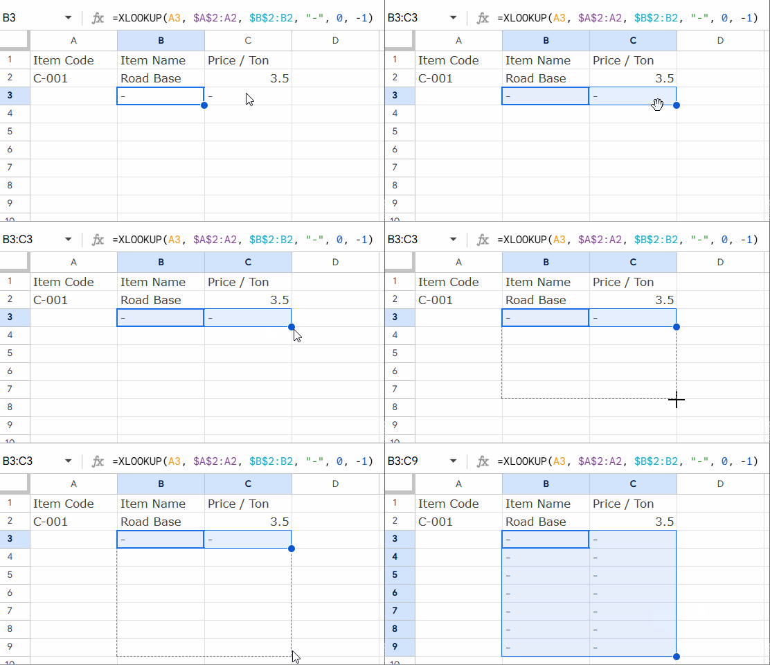
Start by entering your first full record manually in row 2 (with headers in row 1). After that, set up the formulas to pull values from earlier rows when a matching code appears.
- Step 1: Use this formula in cell B3 (for Item Name)
=XLOOKUP(A3, $A$2:A2, $B$2:B2, "-", 0, -1)- Step 2: In cell C3 (for Price), enter:
=XLOOKUP(A3, $A$2:A2, $C$2:C2, "-", 0, -1)- Step 3: Drag the formulas down
Select B3 and C3, and drag the fill handle down through the rows where you plan to enter more item codes.

Now whenever you enter a code in column A (like C-001 again), the name and price will auto-populate from the rows above if that code already exists.
How This Formula Works
Let’s break it down:
=XLOOKUP(A3, $A$2:A2, $B$2:B2, "-", 0, -1)- A3: The item code you’re currently entering
- $A$2:A2: The lookup range — all rows above the current row
- $B$2:B2: The return range — must match the lookup range in height
- “-“: If there’s no match above, return a dash (you can use
""for blank) - 0: Exact match required
- -1: This searches from the bottom up, so it finds the most recent match above
This setup ensures that if you repeat a product code, its details from the most recent occurrence above will be pulled in automatically.
Tip: Handling No Match Above
If the product code is entered for the first time, XLOOKUP won’t find a match. It’ll return "-" (or blank if you modified it). That’s your cue to manually enter the details, and from that point on, the formulas will handle the rest.
Why Use This Method?
This is useful when:
- You’re repeatedly entering product or item codes
- You want to reduce redundant typing
- You want to keep data consistent by copying previously used details
It’s also much cleaner than using scripts or extra helper columns.
That’s it! With just a couple of formulas, you can set up a smart data entry system that auto-populates a row from above when a value repeats. If you’re handling inventory, purchase logs, or any type of repeated data entry, this trick will save you time and effort.


