This post explains how to write a dynamic array formula to multiply every two columns in Google Sheets. There are two solutions.
Where does this type of multiplication come into use?
If the (purchase or sell) prices of items keep changing, you may find this type of calculation worthy.
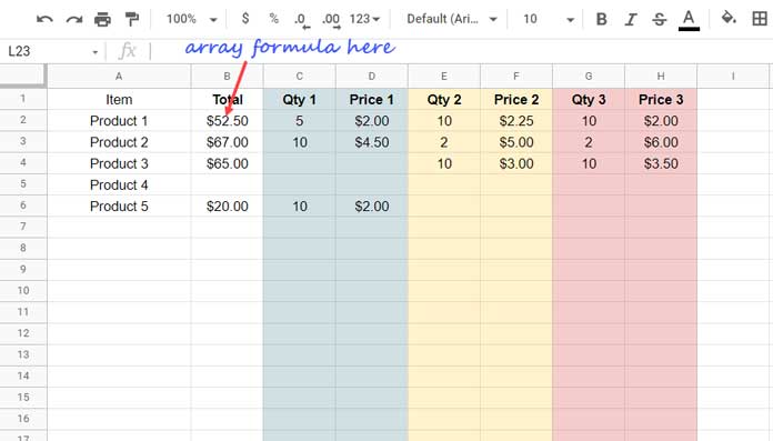
For example, see this sample data (purchase).

There are five products in column A, and you have the break-up of their purchase.
Let’s take one item, i.e., “Product 1”. The total quantity of it is 5+10+10=25.
Instead of specifying 25 in cell C2, I have distributed them in three columns because their purchase prices were different every time.
In this case, to get the total purchase amount, we can use the following formula in cell B2.
OPTION # 1 (NON-ARRAY)
=C2*D2+E2*F2+G2*H2Alternatively, we can use the MULTIPLY function as below.
OPTION # 2 (NON-ARRAY)
=multiply(C2,D2)+multiply(E2,F2)+multiply(G2,H2)Array Formula to Multiply Every Two Columns and Total – Non Dynamic
I know you are familiar with these two types of formulas. But what about an array formula to multiply every two columns and total as above in Google Sheets.
Google Sheets offers the ArrayFormula function to convert such formulas to expand in rows.
Empty B2:B. Then try either of the below array formulas in cell B2 to multiply every two columns in the range and total them.
OPTION # 1 (ARRAY)
=ArrayFormula(IFERROR(1/(C2:C*D2:D+E2:E*F2:F+G2:G*H2:H)^-1))OPTION # 2 (ARRAY)
=ArrayFormula(IFERROR(1/(multiply(C2:C,D2:D)+multiply(E2:E,F2:F)+multiply(G2:G,H2:H))^-1))Please note that the highlighted parts are optional.
If the multiplication formula returns zeros, it converts them into errors and thus makes them blank.
So in an open column range, the highlighted parts make the output more reader-friendly.
In Excel in Office 365, we can use the LET function for that. But at present, Google Sheets doesn’t have that enticing function.
So we use the above workaround, which is popular among Google Sheets’ Product Experts.
The above formulas, of course, return an array result.
But no way as a dynamic array formula as you may require to add new columns within it manually.
Array Formula to Multiply Every Two Columns and Total – Dynamic
Generic Formula:
ArrayFormula(mmult(multiply(filter(Qty_Columns),filter(Price_coluns)),{1;1;1}))Let’s follow the above generic (dynamic array) formula to multiply every two columns and total in Google Sheets.
There are two main parts and one sub-part.
- MULTIPLY.
- FILTER.
- MMULT.
Here are the details.
1. Virtual Arrays within the MULTIPLY Functioin
We can use virtual arrays within the MULTIPLY function to return a matrix output.
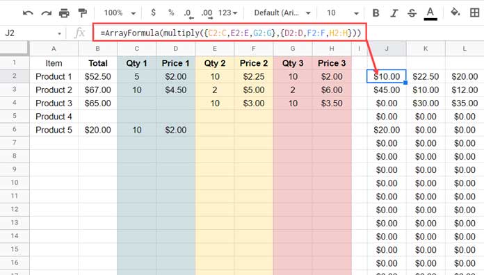
The following formula will return the output of C2:C*D2:D, E2:E*F2:F, and G2:G*H2:H in three columns.
STEP_1 FORMULA (NON DYNAMIC)
=ArrayFormula(multiply({C2:C,E2:E,G2:G},{D2:D,F2:F,H2:H}))
We require a dynamic array formula to multiply every two columns in Google Sheets.
So instead of specifying column ranges as above, we require to use the whole range C2:H. The FILTER comes into use here.
1.1. Filtering Factors
The MULTIPLY function has two arguments, and they are factor1 and factor2.
Syntax: MULTIPLY(factor1, factor2)
factor1 – {C2:C,E2:E,G2:G}
factor2 – {D2:D,F2:F,H2:H}
We can use the FILTER function to extract the factors with the help of the ISODD and ISEVEN functions.
factor1- filter(C2:H,isodd(column(C1:H1)))
factor2 – filter(C2:H,ISEVEN(column(C1:H1)))
These help us to make our step_1 formula dynamic. Here it is.
STEP_1.1 FORMULA (DYNAMIC)
=ArrayFormula(multiply(filter(C2:H,isodd(column(C1:H1))),filter(C2:H,ISEVEN(column(C1:H1)))))We have coded the dynamic array formula to multiply every two columns in Google Sheets. The totaling part is only left.
I mean, the outputs are in three columns. We require to total them. Let’s use MMULT for that.
2. MMULT – Total Multiplied Columns
We require just one more step to add the output row-wise.
For that purpose, we can try different functions that include QUERY, MMULT, DSUM, and SUMIF in Google Sheets. Here are two related links.
- QUERY and MMULT – How to Sum Each Row in Google Sheets.
- DSUM and SUMIF – How to Use the Sumif Function Horizontally in Google Sheets.
Here I am using MMULT.
Syntax:- MMULT(matrix1, matrix2)
matrix1 – STEP_1.1 FORMULA (DYNAMIC)
matrix2 – =ArrayFormula(sequence(COLUMNS(C1:H1)/2)^0)
There are six columns involved in the multiplication calculation as the range is C1:H.
So the STEP_1.1 FORMULA (DYNAMIC) output will be in three columns. Please see image # 2 above.
Since STEP_1.1 FORMULA (DYNAMIC) is matrix1, we require to specify the array {1;1;1} as matrix2 in MMULT to add the columns.
That means if the outputs are in three columns, we require 1 column containing three rows. The SEQUENCE-based matrix2 formula dynamically returns that.
Here is the final formula (for cell B2).
=arrayformula(IFERROR( 1 / mmult(MULTIPLY(filter(C2:H,isodd(column(C1:H1))),filter(C2:H,ISEVEN(column(C1:H1)))),sequence(COLUMNS(C1:H1)/2)^0) ^ -1))This way we can code an array formula to multiply every two columns and total in Google Sheets.
Additional Tips and Query Alternative
I know you might use the above formula in a different range rather than C2:H.
No issue, you can make the formula work by adjusting the range references in the formula.
But, you must make sure that the total number of columns in the multiplication range is even.
In the above formula, it’s 6 (C2:H), which satisfies this condition.
Here is an additional formula, and here also, the above condition is applicable.
If you want, you can replace the above solution in cell B2 with the following QUERY alternative. It is also dynamic!
=ArrayFormula(iferror(1/query(query({n(C2:H)},"Select "®exreplace(REGEXREPLACE(textjoin("*",true,"Col"&sequence(1,columns(C1:H1))),"(.*?\*){2}","$0+"),"\*\+","+")),"offset 1",0)^-1))Do you want to learn this formula too? If so, here are the quick tips.
We can shorten the above Query as below. The below-highlighted part (non-dynamic) replaces the above bold part (dynamic).
=ArrayFormula(iferror(1/query(query({n(C2:H)},"Select Col1*Col2+Col3*Col4+Col5*Col6"),"offset 1",0)^-1))How to make the highlighted part dynamic? To learn that, you can follow this tutorial – How to Replace Every Nth Delimiter in Google Sheets.
That’s all. Thanks for the stay. Enjoy!


