


")


")

")
")
 in Excel & Google Sheets")


Creating an amortization schedule in Google Sheets is straightforward with built-in financial functions like PMT, PPMT, and IPMT. But if you want to pay off your loan early by making extra principal payments, you’ll need a more dynamic approach.
In this tutorial, you’ll learn:
- How to build a basic amortization schedule in Google Sheets
- How to customize it to include extra principal payments to reduce interest and pay off early
⚠️ These schedules assume a constant interest rate and fixed periodic payments.
1. Amortization Schedule in Google Sheets Using Built-in Functions
Google Sheets offers powerful financial functions that make it easy to calculate a loan repayment schedule. Whether your payments are weekly, fortnightly, monthly, or quarterly, the method remains mostly the same.
Let’s walk through creating a monthly amortization schedule step by step.
Required Inputs
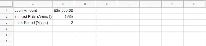
- Loan Amount
- Annual Interest Rate
- Loan Term in Years
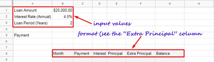
Step 1: Set Up Input Fields
Create a small input section with the following layout:
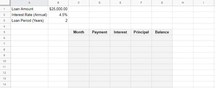
Step 2: Build the Amortization Table Format
Set up a table with the following columns:
- Period
- Payment
- Interest
- Principal
- Balance
Step 3: Enter Formulas
Number of Periods (C6):
=SEQUENCE(24)This generates numbers 1 to 24 for 24 months (2 years × 12).
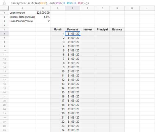
Monthly Payment Using PMT
Formula in D6:
=ArrayFormula(IF(LEN(C6:C), -PMT($B$2/12, $B$3*12, $B$1), ))What it does:
$B$2/12: Monthly interest rate$B$3*12: Total number of months$B$1: Loan amount- Returns constant monthly payments across 24 periods
💡Learn more about the PMT function in Google Sheets — calculates the payment for a loan based on constant payments and interest rate.
Interest Payment Using IPMT
Formula in E6:
=ArrayFormula(IF(LEN(C6:C), -IPMT($B$2/12, C6:C29, $B$3*12, $B$1), ))What it does:
- Calculates the interest portion for each payment period
💡Learn more about the IPMT function in Google Sheets — calculates the interest portion of a payment for a given period of a loan.
Principal Payment Using PPMT
Formula in F6:
=ArrayFormula(IF(LEN(C6:C), -PPMT($B$2/12, C6:C29, $B$3*12, $B$1), ))What it does:
- Calculates the principal portion for each period
- Alternatively, use
=ArrayFormula(D6:D-E6:E)
💡Learn more about the PPMT function in Google Sheets — calculates the principal portion of a payment for a given period of a loan.
Remaining Loan Balance
Formula in G6:
=ArrayFormula($B$1 - SCAN(0, F6:F29, LAMBDA(acc, val, acc + val)))What it does:
- Uses SCAN to cumulatively subtract principal paid and calculate remaining balance
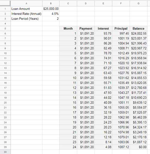
Finished Table
Now your amortization schedule is complete with 24 months of loan breakdown by principal, interest, and balance.
Adjusting for Weekly, Fortnightly, or Quarterly Payments
To change your payment frequency:
- Weekly Rate = Annual Interest Rate / 52
- Fortnightly Rate = Annual Interest Rate / 26
- Quarterly Rate = Annual Interest Rate / 4
Also update the number of periods:
- Multiply years by 52 (weekly), 26 (fortnightly), or 4 (quarterly)
Update all formulas accordingly:
=PMT(Interest Rate ÷ Frequency, Periods × Frequency, Loan Amount)2. Amortization Schedule with Extra Principal Payments in Google Sheets
If you’re making extra payments, you’ll need to modify your amortization logic manually. Google’s financial functions (except PMT) won’t support this natively.
Inputs
Use the same loan input fields, but add a new column for extra payments.
Let’s assume:
- Monthly payment of $500 extra
- This reduces your repayment term from 24 months to 17
Manually enter numbers 1 to 17 in B10:B26.
Step-by-Step Formulas
PMT Calculation in B5:
=-PMT(B2/12, B3*12, B1)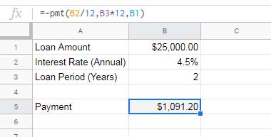
Initial Balance in G9:
=B1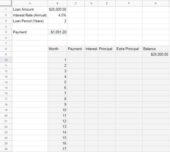
Payment with IF Logic (Cell C10):
=IF($B$5<=G9, $B$5, G9 + (G9 * $B$2/12))Drag this formula down from C10 to C26.
What it does:
- Keeps PMT fixed until the balance is lower than PMT
- In final period, it pays off the remaining balance and interest
Interest Payment (D10):
=IF(LEN(C10), G9 * $B$2/12, 0)Drag down from D10 to D26.
What it does:
- Calculates interest based on the balance from previous row
Principal Payment (E10):
=IF(LEN(C10), MIN(C10 - D10, G9), 0)Drag down from E10 to E26.
What it does:
- Subtracts interest from payment
- Ensures it doesn’t exceed remaining balance
Extra Payment (F10:F25):
Enter $500 in each row manually.
Balance (G10):
=IF(G9 > 0, G9 - E10 - F10, 0)Drag down from G10 to G26.
What it does:
- Reduces balance by both principal and extra payments
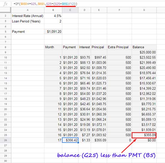
Your table will dynamically reduce the loan balance each month and automatically stop once the loan is paid off. By the 17th month, the balance should hit zero — saving you interest and reducing your loan term.
Conclusion
Using Google Sheets, you can easily build an amortization schedule and simulate early payoff with extra principal payments. It’s a great way to visualize how making small additional contributions can reduce your loan term and save on interest.
If you’re interested, feel free to explore the sample Google Sheet I’ve shared.