To add a column header to array formula results, you can use functions like VSTACK, HSTACK, or curly braces {} in Google Sheets. The method you choose depends on whether your array result is vertical (one column), horizontal (one row), or two-dimensional (a full table).

Mastering this is also helpful when you’re hardcoding criteria in database functions, as they require field labels to be included along with the criteria.

Let’s go over how to add column headers to ArrayFormula results in Google Sheets.

Add Column Header to One-Dimensional ArrayFormula Results

Several functions in Google Sheets return a single column or row. If your array formula outputs a single column (vertical array), you can add a header using VSTACK:

=VSTACK("Salary", ArrayFormula(B2:B * C2:C))

Alternatively, you can use curly braces:

={"Salary"; ArrayFormula(B2:B * C2:C)}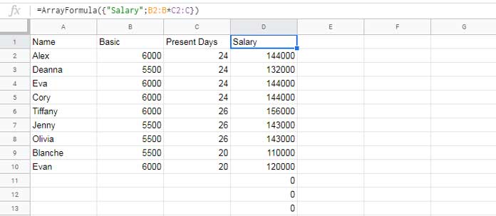

Add Field Label to the First Row of a Single Column ArrayFormula

Just replace ArrayFormula(B2:B * C2:C) with your actual array formula and "Salary" with your desired field label.

Tip: When you add a header row, the formula should be placed one row above where you’d usually place it. Otherwise, Google Sheets may try to output extra blank rows at the bottom, which can slow down performance.

What about adding a header to a horizontal array?

Here’s an example. Suppose you’re looking up the date 24/05/2019 in column A and returning values from B2:D.

=XLOOKUP(DATE(2019, 5, 24), A2:A, B2:D)

To add the label “Result:”, use the HSTACK function with the array formula as follows:

=HSTACK("Result:", XLOOKUP(DATE(2019, 5, 24), A2:A, B2:D))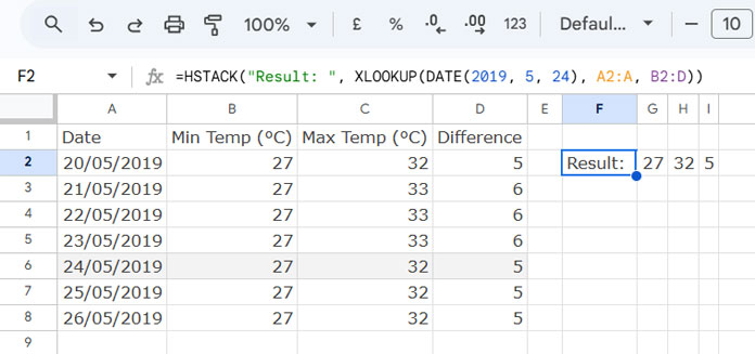

Or with curly braces:

={"Result:", XLOOKUP(DATE(2019, 5, 24), A2:A, B2:D)}

That’s how you add a header to a one-dimensional array formula result in Google Sheets.

Add Column Header to Two-Dimensional ArrayFormula Results

Let’s say you want to filter data in A1:D where the amount in column B equals 5500:

=FILTER(A1:D, B1:B = 5500)

This will return a 4-column table if there’s a match, or #N/A if there isn’t.

To add column headers, use a combination of VSTACK and HSTACK:

=VSTACK(HSTACK("Name", "Basic", "Present Days", "Salary"), FILTER(A1:D, B1:B = 5500))

Here:

• HSTACK creates a header row.
• VSTACK stacks the header on top of the filter result.

You can also use curly braces:

={"Name", "Basic", "Present Days", "Salary"; FILTER(A1:D, B1:B = 5500)}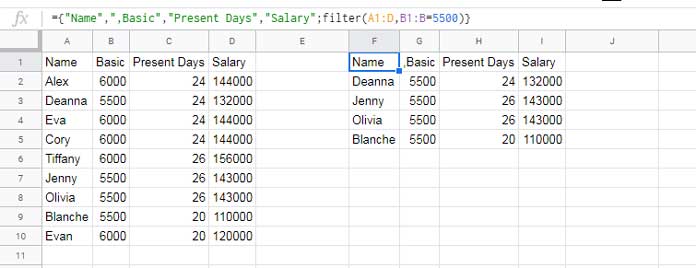

Add Field Label to a Multi-Column ArrayFormula Result

Both these methods behave differently when the FILTER formula returns #N/A:

• The VSTACK + HSTACK method still shows the headers, with a row of #N/A below. You can wrap it with IFNA to suppress that:

=IFNA(VSTACK(HSTACK("Name", "Basic", "Present Days", "Salary"), FILTER(A1:D, B1:B = 5500)))

• The curly braces method throws a #VALUE! error because it tries to combine arrays of different sizes. You can fix that by wrapping it with IFERROR:

=IFERROR({"Name", "Basic", "Present Days", "Salary"; FILTER(A1:D, B1:B = 5500)})

In summary:

• VSTACK + HSTACK always shows headers (even if the result is empty).
• Curly braces will only work if the result isn’t empty—unless wrapped with IFERROR.

Important

When adding headers to array formula results, place the formula one row above where you’d normally place it (if you weren’t using a header). This prevents Sheets from pushing extra blank rows to the bottom, which could impact performance.

Conclusion

If you’re using the QUERY function, it automatically includes a header row.

• If your source data has no header, use the label clause to insert one.
• If the source already has a header, you can keep or override it using label.

In such cases, you don’t need the approaches discussed above.

Resources

• Column Terminology in Google Sheets: Headings, Labels & Names
• Understand the Label Clause in Google Sheets Query
• Mastering Criteria in Database Functions in Google Sheets