
 in Google Sheets")

")


")


")


To find the last business day of a date or the current month in Excel, use WORKDAY.INTL and EOMONTH functions.
This can be useful in many scenarios such as raising monthly invoices (running account bills) on the last business day, financial reporting, payroll preparation, etc.
Before diving into the formula and steps, it’s important to note how weekends are defined within the formula in Excel.
By default, it assumes Saturdays and Sundays are weekends. This setup determines the last business day of a given month based on these traditional weekend days.
Traditional Weekends (Saturday and Sunday) and Control
The formula that returns the last business day of a month in Excel uses seven 0s and 1s to specify the weekend configuration.
For the traditional weekend, it will be “0000011”, where a zero means that the day is a workday, and a one means that the day is a weekend.
In this sequence, the first number represents Monday, and the last number represents Sunday.
Controlling Weekends: In most Middle Eastern countries, the weekends are typically Friday and Saturday. In that case, you can control the weekends in the formula by using “0000110”.
Formula to Find the Last Business Day of a Month in Excel
Enter any date in cell A1. If you want to find the last business day of the current month, enter =TODAY() in cell A1.
In cell B1, enter the following formula:
=WORKDAY.INTL(EOMONTH(A1, 0)+1, -1, "0000011")Navigate to cell B1 if it is not already the active cell.
On the Home tab, within the Number group, select Short Date or Long Date from the drop-down menu.
You will get the last business day of the date specified in cell A1.
How do I check it?
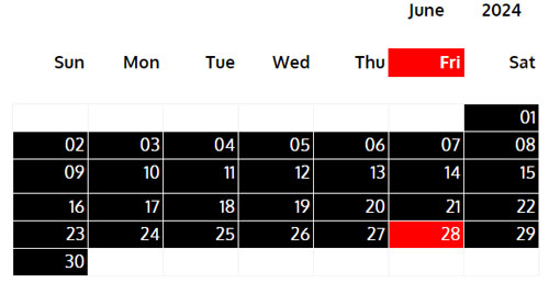
Let’s enter the date 2024-06-10 in cell A1. The formula will return the last business day as 2024-06-28.
Interesting Fact:
If the entered date falls after the last business day of that month, it will typically be a weekend. Even in that scenario, the formula will still return the last business day. For example, if the date is 2024-06-29, the formula will return 2024-06-28.
Formula Breakdown
The EOMONTH function here finds the last day of the month for the date in cell A1.
Next, we add 1 to this result to obtain the first day of the next month.
The WORKDAY.INTL function is then employed, which returns the date value of the date obtained from the previous step, adjusted before or after a specified number of workdays. This function uses custom weekend parameters specified as “0000011”, with the number of workdays set to -1. This setup ensures that the formula accurately identifies and returns the last business day of the specified date.
Since the output of the formula is a date value represented as a serial number, it is formatted back into a date format for clarity and usability.
Why Does the Formula Return 31 as the Last Business Day?
The formula may return the date serial number 31, which corresponds to January 31, 1900, when formatted to a date, if the cell is empty.
An empty cell is interpreted as 0 (January 0, 1900), and 31 (January 31, 1900) is considered the last business day in that month.
If you want to return an empty string (“”) instead of 31 when the cell is empty, modify the formula as follows:
=IF(A1="","",WORKDAY.INTL(EOMONTH(A1,0)+1,-1,"0000011"))The IF logical function tests whether A1 is blank. If it evaluates to TRUE (A1 is empty), it returns an empty string (“”). Otherwise, it returns the last business day of the month.