")
")


")


")

")
")
 in Excel & Google Sheets")


In Excel for Microsoft 365 or versions 2021 and above, we can use the XLOOKUP function to retrieve the first and last non-blank values in a row.
This is particularly useful for horizontally aligned data such as daily, weekly, or monthly sales across rows, attendance records, test scores, etc.
For example, if we have weekly sales data across rows in B2:H2 and want to find the first and last sales values, we can use the following XLOOKUP formulas.
Sample Data in B1:H7:
| Sun | Mon | Tue | Wed | Thu | Fri | Sat |
| 1 | 5 | 6 | 7 | |||
| 5 | 2 | |||||
| 5 | 10 | |||||
| 0 | ||||||
| 10 | 5 | |||||
| 20 | 30 | 16 |
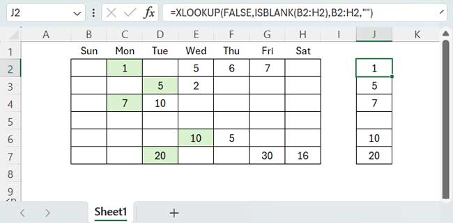
XLOOKUP in Excel for Finding the First Non-Blank Value in a Row
In the data above, you can use the following XLOOKUP formula in cell J2 to get the first non-blank value in that row.
=XLOOKUP(FALSE,ISBLANK(B2:H2),B2:H2,"")Then drag the J2 fill handle down to J7 to apply the formula to each row in the range.
Formula Explanation
The formula follows the XLOOKUP syntax:
=XLOOKUP(lookup_value, lookup_array, return_array, [if_not_found], [match_mode], [search_mode]) In the formula, we have used the following arguments corresponding to each parameter:
lookup_value:FALSE(The value to search in thelookup_array)lookup_array:ISBLANK(B2:H2)(returns FALSE wherever values present in B2:H2 and TRUE otherwise)return_array:B2:H2(the value to return from the column wherelookup_valueis first found in thelookup_array)if_not_found:""(return null if no match is found)match_mode: omitted, 0 by default (exact match of thelookup_value)search_mode: omitted, 1 by default (search from left to right)
In short, XLOOKUP searches for FALSE in the following array:
{TRUE, FALSE, TRUE, FALSE, FALSE, FALSE, TRUE}
and returns the corresponding value from the second column in the range B2:H2.
This helps us find the first non-blank value in a row in Excel using XLOOKUP.
XLOOKUP in Excel for Finding the Last Non-Blank Value in a Row
XLOOKUP can look up a value from right to left in a horizontal range in Excel.
With minimal changes to the above formula, we can find the last non-blank value in a row in Excel.
Formula:
=XLOOKUP(FALSE,ISBLANK(B2:H2),B2:H2, "",0, -1)Enter this formula in cell L2 and drag it down through the desired range.
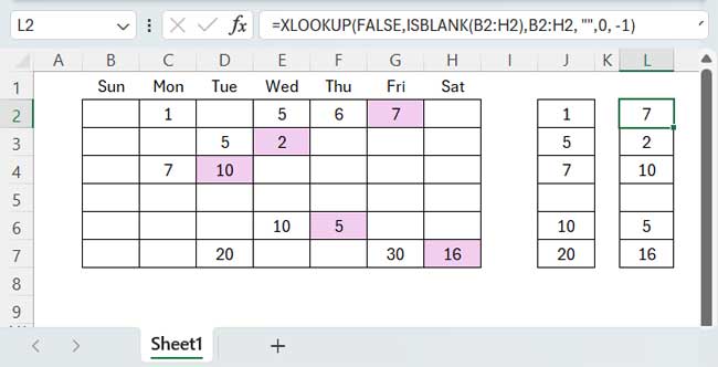
The logic of the formula is exactly the same as the previous one. Here, we additionally specified the last two parameters:
match_mode:0(exact match)search_mode:-1(search from right to left)
Applying Lambda to Spill Formulas Down
Above, we dragged the fill handle of the formulas in cells J2 and L2 down to apply them across the entire range.
If you prefer the formulas to automatically fill down from the first row below the header, using them within an Excel table will achieve this automatically.
However, if you use a range as shown above, you may want to apply the BYROW lambda function to spill the formulas down.
To get the first non-blank value of each row, use the following BYROW formula in cell J2, provided J2:J7 is empty:
=BYROW(B2:H7, LAMBDA(val, XLOOKUP(FALSE,ISBLANK(val),val,"")))Syntax of the BYROW function:
BYROW(array, function)Here, the array is the range B2:H7.
The BYROW function applies the custom lambda function to each row of the array. The lambda function is defined as:
LAMBDA(val, XLOOKUP(FALSE,ISBLANK(val),val,""))This lambda function uses XLOOKUP to find the first non-blank value in each row.
To return the last non-blank value in each row, use the following formula in cell L2, provided L2:L7 is blank:
=BYROW(B2:H7, LAMBDA(val, XLOOKUP(FALSE,ISBLANK(val),val,"",0, -1)))