
")

")
")


")


")


Searching for multiple keywords in a cell is one of the most common tasks in Excel, and dynamic arrays have made it much simpler.
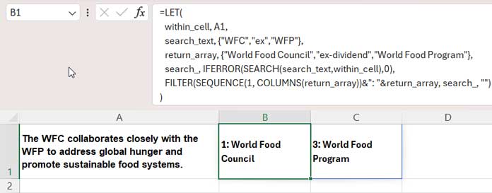
For example, consider the following text in cell A1: “The WFC collaborates closely with the WFP to address global hunger and promote sustainable food systems.“
How do we search for the keywords “WFC,” “ex,” and “WFP” in cell A1 and return 1 and 3 or “1. World Food Council” and “3. World Food Programme” respectively? Because the first and third keywords are available in cell A1.
You can follow the approach below if you are using Microsoft 365 or Excel versions that support dynamic array functions such as LET and FILTER. The LET function is optional, though we have used it to improve the formula’s efficiency by avoiding repeated calculations. It also enhances the overall readability of the formula.
Excel Formula to Search For Multiple Keywords in a Cell
You can utilize the following formula to search for multiple keywords in cell A1 and return assigned values.
=LET(
   within_cell, A1,
   search_text, {"WFC", "ex", "WFP"},
   return_array, {"World Food Council", "ex-dividend", "World Food Program"},
   search_, IFERROR(SEARCH(search_text, within_cell), 0),
   FILTER(SEQUENCE(1, COLUMNS(return_array))&": "&return_array, search_, "")
)
Where:
{"WFC","ex","WFP"}represents the multiple keywords to search in cell A1.{"World Food Council","ex-dividend","World Food Program"}represents the corresponding texts to return.
When using this Excel formula to search for keywords in a cell, replace the values in these two arrays. Both arrays should have an equal number of values.
Please see the formula and output in the screenshot below:
Here are two important changes you can make to the formula to customize the output.
Customization #1:
If you don’t want to return any text and only want the sequences of matches like 1 and 3, remove the &": "&return_array part of the formula.
Output: {1, 3} indicates the first and third keywords match in the sentence.
Customization #2:
If you want the result without the sequence number prefix, remove the SEQUENCE(1, COLUMNS(return_array))&": "& part of the formula.
Output: {World Food Council, World Food Program}
Can I Add Case Sensitivity to the Multiple Keyword Search?
Yes, you can!
Sometimes, case-sensitivity matters in keyword searches in Excel when you want to distinguish between uppercase and lowercase letters in the keywords.
For example, if you’re searching for the keyword “PW123#xy”, which is a password, and your text contains “pw123#xy” or “PW123#XY”, a case-sensitive search would only match “PW123#xy” and not the variations with different capitalization.
For case-sensitive multiple-keyword searches in Excel, you need to make one modification in the formula.
Substitute the function SEARCH with FIND. No other changes to the formula are required. Both share similar syntax; the only distinction is that SEARCH is case-insensitive, whereas FIND is case-sensitive.
Formula Explanation
Here is the key part of the multiple-keyword search formula: IFERROR(SEARCH(search_text, within_cell), 0)
Where the search words (search_text) are {"WFC", "ex", "WFP"} and the cell to search within (within_cell) is A1. We have utilized the LET function to define these two names: search_text and within_cell.
So, what happens here? The above formula is a multiple-keyword search formula that returns either the matching position or 0. In this case, it will return the array {5, 0, 39}. We named this search formula as search_.
Now, here is the formula expression that returns the output: FILTER(SEQUENCE(1, COLUMNS(return_array))&": "&return_array, search_, "")
This formula filters the return array {"World Food Council", "ex-dividend", "World Food Program"} (named return_array) prefixed by their sequence numbers wherever the search_ is greater than 0.