


Using a custom formula in Format > Conditional Formatting, we can highlight named ranges in Google Sheets.
This Google Sheets tutorial provides the formula, steps to add it within the Conditional Formatting panel (dialog box), and an explanation of the formula.
Before delving into how to highlight one or more named ranges, it’s important to consider its implications.
- Using this feature might slow down the sheet. To optimize performance, remove any unused columns and rows from your entire sheet.
- Additionally, be aware that renaming a named range will invalidate the conditional format rule.
- When modifying the range within Data > Named ranges, you may need to insert or delete rows in the sheet to observe the intended highlighting effect (refresh).
For practical demonstration, we will add two named ranges for testing purposes and highlight them with two different colors.
Note: Here, we are highlighting the entire named range area. If you wish to highlight specific cells based on conditions within the named range, please refer to this guide: How to Use Named Ranges in Conditional Formatting in Google Sheets.
Adding Two Named Ranges
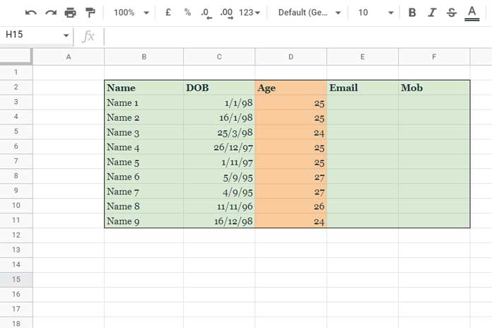
For instance, the range B2:F11 in one of my sheets comprises employee details. I wish to designate this range as “employee” and a specific column within it, namely D2:D11, as “age.”
How can this be achieved?
- Navigate to Data > Named ranges.
- Enter
employeeandB2:F11in the corresponding fields and click on “Done.” - To add the second one, choose “+ Add a range,” input
ageandD2:D11in the respective fields, then click “Done.”
Let’s employ Conditional Formatting to highlight the named ranges “employee” and “age” with distinct colors.
This ensures that when we insert or delete rows or columns in the sheet, the named range and corresponding highlighting will adjust accordingly.
Generic Formula to Highlight Named Ranges in Google Sheets
We will begin with the generic formula:
=ARRAYFORMULA(
     AND(
          AND(
               ROW()>=MIN(ROW(INDIRECT("named_range"))),
               ROW()<=MAX(ROW(INDIRECT("named_range")))
          ),
          COLUMN()>=MIN(COLUMN(INDIRECT("named_range"))),
          COLUMN()<=MAX(COLUMN(INDIRECT("named_range")))
     )
)
In this formula, you’ll notice four instances of the string “named_range.” When applying this generic formula to highlight named ranges, ensure to replace these instances with the actual names as needed.
Adding Two Highlight Rules
We now have a generic formula. We want to highlight two named ranges: “employee” and “age.” Let’s add them one by one in the Conditional Format panel. Here are the steps.
Assume you are testing it in the “Sheet1” tab, which has 26 columns and 1000 rows.
Ensure you apply the highlight rules in the range A1:Z1000. This is crucial!
- Go to Format > Conditional Formatting.
- Enter
A1:Z1000(the entire range in “Sheet1”) in “Apply to the range.” - Select “Custom formula” under “Format rules” and input the generic formula provided above.
- Replace all instances of “named_range” in the generic formula with “employee” (scroll down to see the formula).
- Choose your desired “Formatting style” and select “Done.”
To add the second rule:
- Repeat steps 1 to 5 above.
- In the 4th step, replace “named_range” with “age.”
- In the 5th step, choose a different formatting style.
This process allows us to add conditional format rules to highlight named ranges in Google Sheets.
Highlighting Named Ranges: Anatomy of the Formula
For testing purposes, we will apply the rule that highlights the named range “employee.” Here it is.
=ARRAYFORMULA(
     AND(
          AND(
               ROW()>=MIN(ROW(INDIRECT("employee"))),
               ROW()<=MAX(ROW(INDIRECT("employee")))
          ),
          COLUMN()>=MIN(COLUMN(INDIRECT("employee"))),
          COLUMN()<=MAX(COLUMN(INDIRECT("employee")))
     )
)
We have utilized several Google Sheets functions in the formula. Rather than explaining the role of each function individually, let’s understand them in a combined form.
The INDIRECT function plays a crucial role in the formula since it deals with a string (the name of a range). It is essential to use it when incorporating a named range for highlighting purposes.
When combined with the ROW or COLUMN functions, it provides the respective row and column numbers within this specified range.
=ARRAYFORMULA(ROW(INDIRECT("employee")))The above formula returns the row numbers in the “employee” range, and the following one returns the column numbers.
=ARRAYFORMULA(COLUMN(INDIRECT("employee")))MIN and MAX functions are employed with these two formulas to determine the starting and ending row and column numbers in the “employee” range.
The formulas would return 2, 11, 2, and 6, representing the minimum row number, maximum row number, minimum column number, and maximum column number, respectively.
The highlight rule evaluates each cell in the range A1:Z1000:
- The row number is between 2 and 11, inclusive.
- The column number is between 2 and 6, inclusive.
If the evaluation is TRUE, the formula highlights the cell.
That concludes our discussion on how to highlight named ranges in Google Sheets. Thank you for joining in. Enjoy!