


How many of you know, you can use DPRODUCT for row-wise multiplication of a multi-column array dynamically in Google Sheets.
In this post, you can learn the use of DPRODUCT for the same.
I have already written a couple of tutorials for row-wise array formulas. That includes solutions based on Database functions as well as alternative solutions using either QUERY or MMULT.
For row-wise multiplication also we can use QUERY. You can find that tutorial here – PRODUCT Array Formula for Row-Wise Products in Google Sheets.
But I would rate the following DPRODUCT based solution above QUERY.
Do you know why? Because it is performance enhanced in my test, also simple to code and read.
Let’s go to the formula and example.
DPRODUCT for Row-Wise Multiplication in Google Sheets
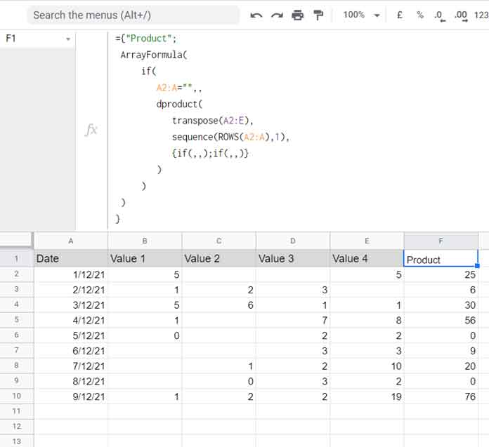
The sample data is a 2-D array with five columns. The first column contains date inputs that we don’t want to include in the multiplication.
Here are the formula, sample data, and the result.
={"Product";
 ArrayFormula(
     if(
        A2:A="",,
        dproduct(
           transpose(A2:E),
           sequence(ROWS(A2:A),1),
           {if(,,);if(,,)}
        )
     )
 )
}
I would rate this formula as the best formula for Row-Wise Multiplication of a 2-D array dynamically in Google Sheets.
The database function is for structured data. Can I use this if my dataset has no field labels and an additional column (date column) as above?
My answer is yes. Let’s learn the formula first.
Formula Explained
One of the best ways to learn the above DPRODUCT formula is to modify the cell range from open to close (infinite to finite). By doing so, we can exclude the use of the below IF test.
if(A2:A="",,Then remove any field label suffixed to the formula.
{"Product";formula_here}Here is the formula after the said two modifications.
=ArrayFormula(
     dproduct(
        transpose(A2:E10),
        sequence(ROWS(A2:A10),1),
        {if(,,);if(,,)}
     )
)
Now let’s understand this DPRODUCT formula.
Syntax: DPRODUCT(database, field, criteria)
Here is how we have used each argument in the formula.
DATABASE: transpose(A2:E10)
Why I have transposed the range A2:E10?
It’s because DPRODUCT is not for Row-Wise Multiplication. It’s for Column-wise multiplication. So we have transposed our range from rows to columns.
FIELD: sequence(ROWS(A2:A10),1)
Our data is spread across nine rows from 1 to 9 and 6 columns from A to E. When we transpose, it becomes nine columns and six rows.
That means we want the row-wise multiplication result from columns 1-9. The above SEQUENCE returns the field numbers 1 to 9 with the help of ROWS.
CRITERIA: {if(,,);if(,,)}
We have no criteria column. But we must specify criteria that at least contain two cells vertically. It can be blank. The above formula does that.
Row-Wise Multiplication Using DPRODUCT in an Unstructured Data
I am unable to use your formula because I don’t have field labels and a criteria column. I am talking about the date column in your data above.
In that scenario, how can I use the above formula for row-wise multiplication in a multi-column array?
Of course, I can. You must understand certain things about the database function use in Google Sheets.
What are they?
All the database functions do require field labels. If you don’t have them in your dataset, you should select any blank row that contains as many columns in the 2-D array.
Here we should select a blank column as we are transposing columns to rows. Here in the below example, that said column is J2:J10.
=ArrayFormula(
     dproduct(
        transpose({J2:J10,B2:E10}),
        sequence(rows(B2:B10),1),
        {if(,,);if(,,)}
     )
)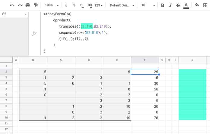
Even if you don’t have any such column to include in the formula, you can consider any column in the source itself. For example, you can replace J2:J10 with B2:B10 also.
That’s all about the row-wise multiplication using DPRODUCT in a 2-D matrix in Google Sheets.
Thanks for the stay. Enjoy.