We can use the PRODUCT function in Google Sheets to return the product of a series of numbers. The product is the result you get when two or more values are multiplied together.
You can also use the * (asterisk) operator to return the product of values, but it’s not always a perfect alternative to the PRODUCT function.
If you’re working with just two values (factor 1 and factor 2), you can use the PRODUCT function, the asterisk operator, or even the MULTIPLY function.
However, when dealing with more values, using the PRODUCT function is the better approach. I’ll explain why shortly.
In this post, you’ll learn how to use the PRODUCT function in Google Sheets effectively. You’ll also find a few helpful tips—like combining the PRODUCT function with FILTER to exclude zeros or apply conditions to a specific range.
Syntax of the PRODUCT Function in Google Sheets
Syntax:
PRODUCT(factor1, [factor2, ...])Arguments:
factor1– The first number, cell reference, or array to include in the multiplication.factor2, …– Additional numbers or ranges to multiply.
You can specify up to 30 arguments directly, but according to the official documentation, the PRODUCT function can actually take an arbitrary number of arguments.
Here are a few examples that make using this handy math function in Google Sheets simple.
Simple Example of Using PRODUCT Function
=PRODUCT(5, 10, 2)The above formula returns 100, which is the same as:
=5 * 10 * 2When you input numbers directly in the formula, there’s little difference between using the PRODUCT function and the asterisk operator. Both are equally easy to write.
However, when the arguments are cell references, the PRODUCT function becomes more practical and readable compared to the asterisk operator.
Below are some practical examples of how to use the PRODUCT function in Google Sheets with different types of ranges:
=PRODUCT(A2:A7)
=PRODUCT(E2:F4)
=PRODUCT(E8:E10, F8:F10)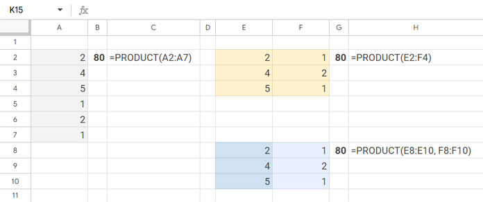
PRODUCT Function Behavior in Google Sheets
Note:
- The PRODUCT function in Google Sheets will ignore text strings, Boolean values (
TRUE/FALSE), and blank cells in the array. - However, it will include date and time values in the calculation.
- Also, the input array doesn’t need to be uniform in shape.
Why MULTIPLY or Asterisk Isn’t a Full Alternative
If you reviewed the screenshot examples, you’ll notice why the asterisk operator isn’t a practical replacement for the PRODUCT function in every scenario.
For example, here’s how the formula in cell B2—=PRODUCT(A2:A7)—would look if rewritten using the asterisk operator:
=A2 * A3 * A4 * A5 * A6 * A7As the number of values increases, this method becomes unwieldy and harder to maintain.
The MULTIPLY function is another option, but it’s designed only for:
- Multiplying two numbers, or
- Multiplying one array by another (element-wise).
Here are two examples:
Examples Comparing MULTIPLY, Asterisk, and PRODUCT Formulas
Example 1:
=MULTIPLY(5, 10)Result: 50
Example 2:
| A | B | C |
|---|---|---|
| Quantity | Rate | Amount |
| 5 | 10 | 50 |
| 4 | 20 | 80 |
| 6 | 30 | 180 |
In cell C2, you can use either of the following formulas (but not PRODUCT):
Formula 1:
=ArrayFormula(MULTIPLY(A2:A4, B2:B4))Formula 2:
=ArrayFormula(A2:A4 * B2:B4)So, while MULTIPLY works in array scenarios, it doesn’t replace PRODUCT when you need to multiply many values flexibly.
PRODUCT Function with FILTER in Google Sheets (Conditional Product)
Besides numbers and cell references, the arguments in the PRODUCT function can include expressions. That means you can pass another function as an argument.
Let’s say you want to calculate the product of values between 1 and 3 (inclusive) in the range A1:A. You can use the FILTER function with PRODUCT like this:
=PRODUCT(FILTER(A1:A, A1:A >= 1, A1:A <= 3))Similarly, if you want to exclude zeros, use:
=PRODUCT(FILTER(A1:A, A1:A > 0))This approach makes the PRODUCT function in Google Sheets even more powerful, especially in conditional scenarios.
Additional Tip: PRODUCT Array Formula for Row-Wise Products in Google Sheets
Sometimes, you might want to calculate the product across rows—that is, multiply values horizontally rather than down a column.
Let’s take this sample data in columns A to D:
| Item | Qty | Units/Box | Rate |
|---|---|---|---|
| LED COB Light | 50 | 5 | $6.00 |
| LED Spot Light | 2 | 5 | $29.00 |
| LED Chandelier Ring | 1 | 1 | $90.00 |
For the first item, the total value is:
50 boxes × 5 units per box × $6 per unit = $1,500
You can calculate the row-wise total in two ways:
Option 1: Regular Formula (Non-Array)
In cell E2, use either:
=B2*C2*D2or:
=PRODUCT(B2:D2)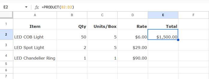
Then drag the formula down to fill the other rows.
Option 2: Array Formula Using BYROW + PRODUCT
If you prefer an array formula that handles all rows at once, use:
=BYROW(B2:D, LAMBDA(row, PRODUCT(row)))This returns the product for each row in the range B2:D.
Note: If you want to return a blank instead of 0 when the row’s product is zero, use this version:
=BYROW(B2:D, LAMBDA(row, LET(total, PRODUCT(row), IF(total=0, ,total))))Why BYROW?
You can’t use the PRODUCT function directly with ArrayFormula for row-wise calculations. But BYROW combined with LAMBDA allows you to apply the PRODUCT function in Google Sheets to each row individually.
Important Note on Blank Cells and PRODUCT vs Asterisk
The behavior of the PRODUCT function differs from using the * operator when cells are blank.
=PRODUCT(5, , 2)→ Returns 10 (ignores blanks)=5 * "" * 2→ Returns 0
That’s one reason why the PRODUCT function in Google Sheets is more reliable than the asterisk operator, especially for row-wise or conditional calculations.
Conclusion
You now know how to use the PRODUCT function in Google Sheets, from simple calculations to advanced use cases like conditional products with FILTER and row-wise multiplication using BYROW. Whether you’re working with direct numbers, arrays, or filtered data, the PRODUCT function remains a reliable and flexible tool for your spreadsheet tasks.