


To get the cell address of a lookup value in Google Sheets, I have three different formulas that you can try. Two of them are based on the CELL function.
There is an info type called “address” in the CELL function. It helps us to return the cell address of a specified cell.
Syntax: CELL(info_type, reference)
Here are two quick examples.
=cell("address",B9)The above formula would return $B$9 (cell address), whereas the following one would return the width of cell A9.
=cell("width",A9)That means the info type matters.
In the above two formulas, B9 and A9 are called cell references.
The CELL function supports an expression (a formula) as a reference instead of a direct reference to a cell.
The above opens the possibility of using the CELL function to return the cell address of a lookup result value in Google Sheets.
How?
We will use one lookup formula as the reference within CELL. I am going to elaborate on that in the below sections.
Formulas to Get the Cell Address of a Lookup Value in Google Sheets
Sample Data:
Here are the different formula options. As mentioned, I have three formulas, as detailed below.
- Two CELL function-based formulas.
- Using Vlookup.
- Using Index-Match
- One IF and SORTN based formula.
CELL Function Based
Let’s start with the Vlookup and CELL combo.
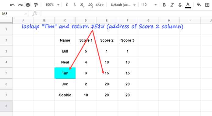
In the above dataset in Google Sheets, I want to lookup the name “Tim” and return the cell address from the “Score 2” column.
The logic here is to use Vlookup to return the lookup value instead of the cell ID and use it as the reference (expression) within CELL.
The following formula will search down “Tim” in C2:F2 (the first column in the array C2:F7) and will return the value (Score 2) from the third column.
=VLOOKUP("Tim",C2:F7,3,0)Just use this as the reference in one CELL formula as below to get the cell address of the lookup value, i.e., “Tim”.
Formula 1:
=cell("address",vlookup("Tim",C2:F7,3,0))Result: $E$5
The Index-Match formula follows the same path. Here we offset a specific number of rows and columns to return the same above Vlookup result. We can use that as a reference in CELL as above.
Here is that reference.
=index(C2:F7,match("Tim",C2:C7,0),3)If we shorten the above formula, it would be as below.
=index(C2:F7,4,3)The Index formula offsets four rows to reach the row that contains “Tim” and three columns to the corresponding “Score 2” column.
Just use Index-Match within CELL similar to Vlookup to get the cell address of the Lookup results in Google Sheets.
Formula 2:
=cell("address",index(C2:F7,match("Tim",C2:C7,0),3))IF and SORTN Based
It is going to be a completely different approach and very simple to understand. You can quickly follow my step-by-step instructions below.
First, we will use a logical IF formula to return the row number that matches the name “Tim”.
=ArrayFormula(if(C2:C7="Tim",row(C2:C7)))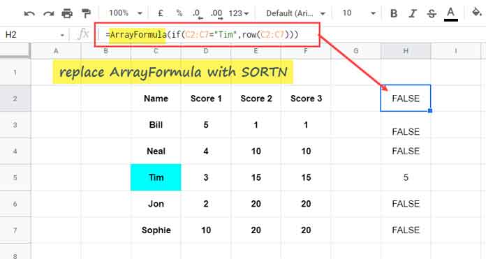
The formula would return values as shown in H2:H7. Replace ArrayFormula with SORTN to get the row number alone.
=SORTN(if(C2:C7="Tim",row(C2:C7)))Prefix the column letter “E” which is the Score 2 column heading with the above output.
Formula 3:
="$E$"&SORTN(if(C2:C7="Tim",row(C2:C7)))That’s all! The above is the third formula to get the cell address of a lookup value in Google Sheets.
Now to one extra goodie.
Cell Address of Lookup Intersection Value in Google Sheets
The above first two formulas (Formula 1 and Formula 2) have one advantage. Because, in that, we have hardcoded the column number. Whereas in the last (third) formula, we have hardcoded a column letter.
Assume we want to lookup and find the cell address of an intersection value. Let’s see what we can do here.
Value to Lookup: “Tim”
Column to Lookup: “Score 1”
In the first two formulas replace the number three with the following horizontal match formula.
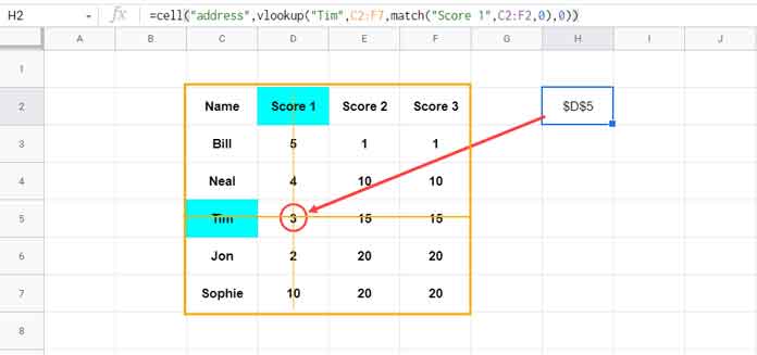
match("Score 1",C2:F2,0)So the Formula 1 will become;
=cell("address",vlookup("Tim",C2:F7,match("Score 1",C2:F2,0),0))and Formula 2 will become;
=cell("address",index(C2:F7,match("Tim",C2:C7,0),match("Score 2",C2:F2,0)))Related: Highlight Intersecting Value in Google Sheets in a Two Way Lookup.
That’s all. Thanks for the stay. Enjoy!