


When you want to see part of a table you can use the built-in Filter menu in Google Sheets. Also, you can create your own drop-down to filter data from a table horizontally or vertically.
The latter will be useful to extract data from a table to a new range and perform additional calculations.
In this Google Sheets tutorial, I am going to share with you how to create a drop-down menu to filter data from not only rows but also from columns.
What more! I have included how to do horizontal and vertical filtering using a drop-down menu.
Here is a visual representation of what I am going to do in this tutorial.
1.Drop-Down Menu to Filter Rows in a Table:
2. Drop-Down Menu to Filter Columns in a Table:
3. Drop-Down to Filter Data From Rows and Columns:
1. Drop Down to Filter Data From Rows in Google Sheets
If you don’t like the filter command in Google Sheets, then there is the Filter function. It offers complete flexibility in filtering.
First, let me show you how to use drop down to Filter data from rows. Then we can move to columns and columns+rows.
How to Create a Drop-Down Menu for Filtering Rows
In the first example, you can find the drop-down in cell E2. How to create that drop-down containing unique values in the range C2:C11?
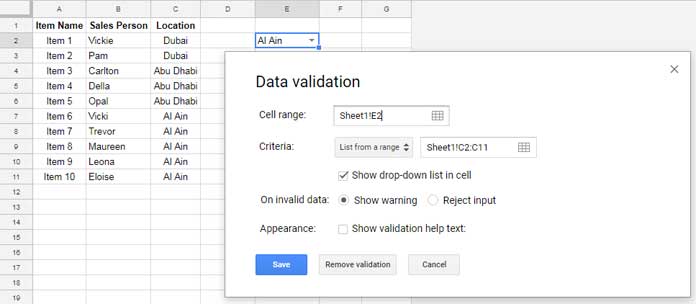
Go to the menu Data > Data Validation. Choose the criteria as “List form a range”. Select the range C2: C11 and click Save.
You May Like: The Best Data Validation Examples in Google Sheets.
Even if there are multiple occurrences of values in the range, Google Sheets data validation rule will only consider the unique values.
Your drop-down menu to Filter data from Rows is ready. Now use this Filter formula in cell E3. That’s all.
=filter(A2:C,C2:C=E2)
2. Drop Down to Filter Data From Columns in Google Sheets
You can search across the first row of a table to find a specific title. Then you can extract the data in that specific column. That is what I have demonstrated in the second example.
How to Create a Drop-Down Menu for Filtering Columns
The drop-down for column filtering is in cell G1. Just follow the above screenshot to create a drop-down menu for filtering in Google Sheets.
Here there is one difference. Choose the criteria as “List form a range” and select the range B1: E1. Yes! The range is obviously different this time.
This time I am not going to use the Filter function. The best formula to filter columns is Query. But what we want is to search the header and then filter.
So here my recommended function is the popular Index-Match combo. Just use this formula in cell G2.
=index(A2:E,0,match(G1,A1:E1,0))
Follow the above instructions to Filter data from columns in Google Sheets.
3. Drop Down to Filter Data From Rows and Columns in Google Sheets
The third example is the compilation of the above two examples. That means there would be two drop-down menus.
The drop-down menu in cell H4 is for filtering rows and the one in H6 for filtering columns.
Actually, As mentioned, I have used two drop-down menus for filtering data from Rows and Columns. But there is only one formula in cell J4.
See that magical formula and details here – Two-way Filter in Google Sheets.
Related Reading:
1. Lookup and Retrieve the Column Header in Google Sheets.
2. Two-way Lookup and Return Multiple Columns in Google Sheets.
If only you had a video for these tutorials it would be useful. But I see no video.