The lack of grouping and subtotal prompts Google Sheets users to try different formula options. This tutorial, how to subtotal up to the first blank cell in a column, is also based on that thought process.
This tutorial covers the following.
1. How to sum up to the first blank cell in Google Sheets.
2. How to subtotal up to the first blank cell in a column in Google Sheets.
What is the difference?
The solution to the second question involves rows that are hidden via filtering, row grouping and hide manually.
As far as I know, the SUBTOTAL() is the one and the only function in Google Docs Sheets that can sum only visible rows.
The function SUBTOTAL is not only for totaling a column that excluding filtered out rows, hidden rows or collapsed row groups. With the help of function_codes, you can use most of the aggregation functions with it.
First, let me show you how to total up to the first blank cell in a column. Then we can go to hidden/grouped/filtered rows.
How to Sum up to the first blank cell in Google Sheets.
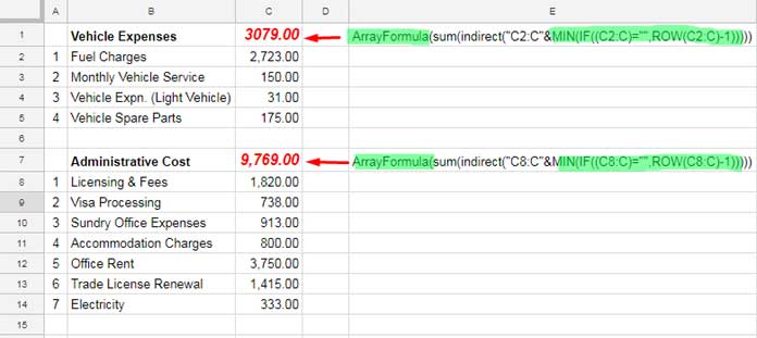
In this example, I want the sum formula (in C1) to total the range C2: C5 since the cell C6 is blank.
Similarly, the second formula in C7 should find the first blank cell in the range C8: C then sums the range C8: C14.

In an earlier Google Docs Sheets tutorial, I have explained how to find the row number of first blank cell in a column. That’s important here.
I am straightaway going to that formula here. If you want to know more about the functioning of it check the tutorial; how to count until a blank row in Google Sheets.
Apply this formula in any blank cell to see what it returns.
=ArrayFormula(MIN(IF((C2:C)="",ROW(C2:C)-1)))
Actually what we want is the sum of the range C2: C5 like;
=SUM(C2:C5)
The above ArrayFormula would return the number 5 in C2: C5. With the help of the function INDIRECT, we can implement that in C2: C as below. I have highlighted the same in the screenshot below.
The formula in cell C1:
=ArrayFormula(sum(indirect("C2:C"&MIN(IF((C2:C)="",ROW(C2:C)-1)))))
The formula for cell C7:
=ArrayFormula(sum(indirect("C8:C"&MIN(IF((C8:C)="",ROW(C8:C)-1)))))
In this formula, the sum range is C8: C14.

If you could understand the above clearly, the next formula to subtotal up to the first blank cell in a column would be easier for you.
How to Subtotal Up to the First Blank Cell in a Column
First, see how this beneficial to you.
Steps:
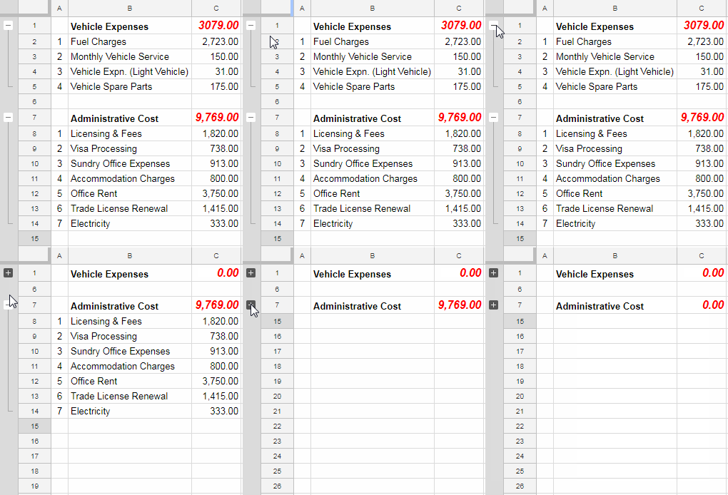
Select the rows 2 to 5, then right click and group. Similarly, select the rows 8 to 14 and group it.
Replace the formula in the cell C1 with the below one.
=ArrayFormula(subtotal(109,indirect("C2:C"&MIN(IF((C2:C)="",ROW(C2:C)-1)))))
Here is the formula in cell C7.
=ArrayFormula(subtotal(109,indirect("C8:C"&MIN(IF((C8:C)="",ROW(C8:C)-1)))))
If you compare these formulas with the earlier sum formula, you can see the difference. There is only one difference, i.e., I have replaced the formula part sum( with the subtotal(109.
Now see this screen capture.

When I collapse the row grouping, the total gets 0 in that group. Expand it again to see the sum of visible rows.
Of course, there is no magic in that. It’s because of the use of the SUBTOTAL function. No doubt the formula would behave similarly with the filtered out or hidden rows.
Similar: Find the Cell Address of a Last Used Cell in Google Sheets.
Hope my attempt to detail you how to subtotal up to the blank cell in Google Sheets has turned beneficial to you. If you like, try sharing it. Thanks for the stay. Enjoy!


Sorry I didn’t add function number that was my mistake. I forget that. Thanks for these tips and tricks 🙂
Welcome!
Hi, how can we do this with subtotal function? I changed it but it didn’t work. Why I need this because I use the filter in my sheet. I want to sum filtered numbers. I read your this post too: https://infoinspired.com/google-docs/how-to-omit-hidden-or-filtered-out-values-in-sum-google-doc-spreadsheet/