Using a dynamic array formula or the FILTER command, we can sort data and keep blank rows in Excel and Google Sheets. While the first approach directly sorts the source data, the formula outputs the results in a new range dynamically. Any future changes in the source will reflect in the formula output, making it a dynamic solution.
I’ve designed a formula that works equally well in both Excel and Google Sheets. In Google Sheets, you need to wrap the formula with the ArrayFormula function. That’s the only difference.
Understanding the Scenario
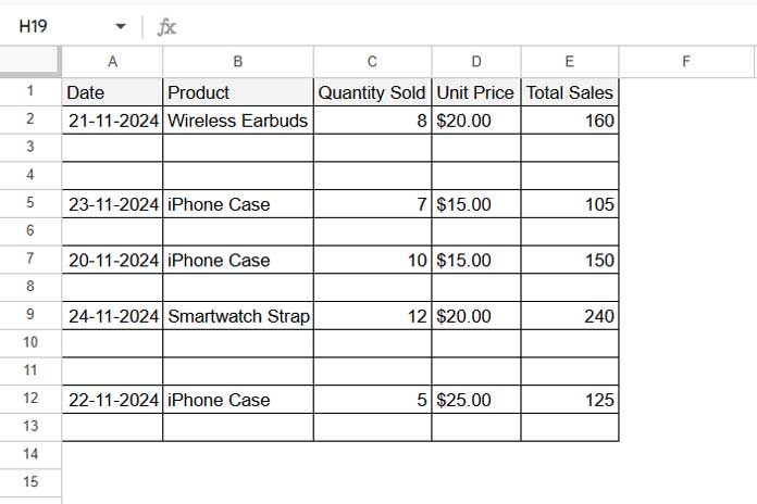
Assume you have sample data in Excel or Google Sheets in the range A1:E13, representing sales data with the headers: Date, Product, Quantity Sold, Unit Price, and Total Sales in A1:E1.

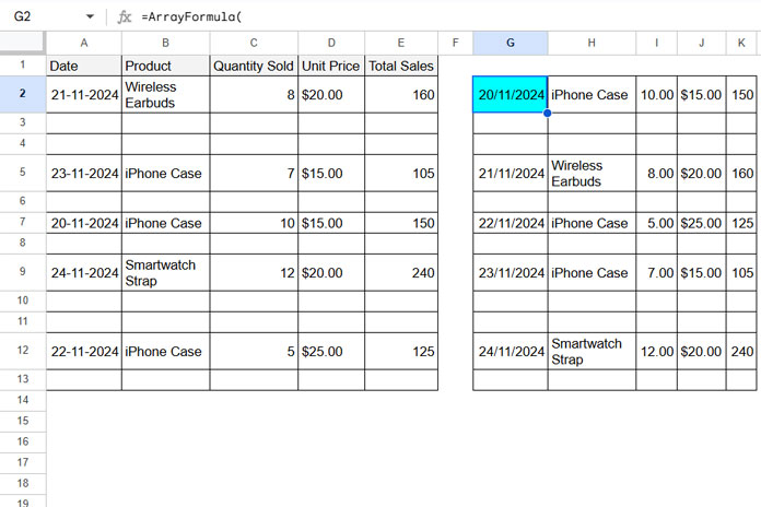
There are blank rows between some records. If you sort the data by any column, the blank rows will move to the bottom. However, you want to sort the data while keeping the blank rows in their original positions. How do you achieve that? This tutorial will guide you.
A Universal Formula to Sort Data and Keep Blank Rows
Formula to Sort Data but Keep Blank Rows
=ArrayFormula(
   LET(
      range, A2:E13,
      bRow, TOCOL(IF(CHOOSECOLS(range, 1)="", ROW(A2:A13),NA()), 3),
      sData, SORT(FILTER(range, CHOOSECOLS(range, 1)<>""), 1, 1),
      dataRow, HSTACK(WORKDAY.INTL(1, SEQUENCE(ROWS(sData)), "0000000", bRow), sData),
      sorted, IFNA(SORT(VSTACK(bRow, dataRow)),""),
      CHOOSECOLS(sorted, SEQUENCE(COLUMNS(range), 1, 2))
   )
)
Important: The formula may convert dates to numeric values. To fix this:
- In Excel: Select the date column in the result range, then go to the Home tab > Number Group > Short Date.
- In Google Sheets: Select the date column, then go to Format > Number > Date.
When using the formula in Excel, remove the ArrayFormula function.

Steps to Adjust the Formula for Your Data
- Replace
A2:E13with your data range (excluding the header row). - Replace
A2:A13with the first column range (excluding the header row). - To sort by a different column, modify the
1, 1part:- For ascending order, keep it as
1, 1(column 1). - For descending order, change it to
1, 0(Google Sheets) or1, -1(Excel).
- For ascending order, keep it as
No additional changes are required. However, if there are no blank rows, the formula may return an error.
Formula Breakdown
Let’s break the formula into parts to understand its functionality.
range:A2:E13
This is the range to sort, excluding the header row.
bRow:TOCOL(IF(CHOOSECOLS(range, 1)="", ROW(A2:A13),NA()), 3)
This part identifies the row numbers of blank rows. The IF function checks if the first column is blank and returns the row number for blank rows or#N/Afor non-blank rows. The TOCOL function removes the#N/Aerrors and returns the blank row numbers as a vertical array. For our sample data, the result is{3; 4; 6; 8; 10; 11; 13}.
sData:SORT(FILTER(range, CHOOSECOLS(range, 1)<>""), 1, 1)
This filters out the blank rows and sorts the remaining data by the first column in ascending order.
dataRow:HSTACK(TOCOL(IF(CHOOSECOLS(range, 1)<>"", ROW(A2:A13),NA()), 3), sData)
This horizontally stacks the row numbers of non-blank rows with the sorted data (sData). For our sample data, the output would look like this:
| 2 | 20/11/2024 | iPhone Case | 10 | $15.00 | 150 |
| 5 | 21/11/2024 | Wireless Earbuds | 8.00 | $20.00 | 160 |
| 7 | 22/11/2024 | iPhone Case | 5.00 | $25.00 | 125 |
| 9 | 23/11/2024 | iPhone Case | 7.00 | $15.00 | 105 |
| 12 | 24/11/2024 | Smartwatch Strap | 12.00 | $20.00 | 240 |
sorted:IFNA(SORT(VSTACK(bRow, dataRow)),"")
This vertically stacksbRow(blank rows) withdataRow(sorted data) and sorts the combined data, ensuring blank rows remain in their original positions.
| 2 | 20/11/2024 | iPhone Case | 10 | $15.00 | 150 |
| 3 | |||||
| 4 | |||||
| 5 | 21/11/2024 | Wireless Earbuds | 8.00 | $20.00 | 160 |
| 6 | |||||
| 7 | 22/11/2024 | iPhone Case | 5 | $25.00 | 125 |
| 8 | |||||
| 9 | 23/11/2024 | iPhone Case | 7 | $15.00 | 105 |
| 10 | |||||
| 11 | |||||
| 12 | 24/11/2024 | Smartwatch Strap | 12 | $20.00 | 240 |
| 13 |
- Final Cleanup:
CHOOSECOLS(sorted, SEQUENCE(COLUMNS(range), 1, 2))
This removes the helper column (row numbers) from the final result, leaving only the sorted data with blank rows intact.
Using the FILTER Command to Sort Data While Keeping Blank Rows Intact
In Excel
- Select the data range A1:E13 (including headers).
- Navigate to the Data toolbar and click on Filter under the Sort & Filter group.
- In the header of the column you want to sort (e.g., Date), click the drop-down and uncheck Blanks.
- Click OK.
- Click the Date drop-down again.
- Sort the column by selecting Sort Oldest to Newest or Sort Newest to Oldest.
- To remove the filter, click Filter again in the Sort & Filter group on the Data toolbar.
In Google Sheets
- Select the data range A1:E13.
- Go to Data > Create a Filter.
- Click the drop-down in the header of the target column (e.g., Date) and uncheck Blanks.
- Click OK.
- Click the Date drop-down again.
- Sort the column by selecting Sort A to Z or Sort Z to A.
- Go to Data > Remove Filter to remove the filter.
Conclusion
Both approaches effectively sort data while keeping blank rows intact. The formula provides a universal and dynamic solution, while the FILTER command is more straightforward for quick sorting tasks.


