


")


")

")
")
 in Excel & Google Sheets")


There isn’t a specific function to calculate the number of days between weekday names (text) in Excel or Google Sheets. This tutorial explains how to achieve this using a formula.
Assume you have data in two columns: one representing the departure weekday (e.g., “Monday”) and the other representing the arrival weekday (e.g., “Friday”). How can you calculate the duration between the departure and arrival weekdays?
Assume that the departure weekday names are in column A, beginning with cell A2, and the arrival weekday names are in column B, starting with cell B2.
Here are the step-by-step instructions for calculating the days between weekday names in Excel and Google Sheets.
Steps
In cell C2, enter the following formula:
=MATCH(A2, {"Monday", "Tuesday", "Wednesday", "Thursday", "Friday", "Saturday", "Sunday"}, 0)This formula matches the text in cell A2 against the array of weekday names and returns its position: 1 for Monday, 2 for Tuesday, and so on up to 7 for Sunday.
In cell D2, enter the following formula:
=MATCH(B2, {"Monday", "Tuesday", "Wednesday", "Thursday", "Friday", "Saturday", "Sunday"}, 0)This formula returns the weekday number for the text in cell B2.
Use the following formula in cell E2 to calculate the duration (number of days) between the weekday names:
=IF(D2>=C2, D2-C2, 7-C2+D2)This formula checks whether the arrival weekday is greater than or equal to the departure weekday. If true, it subtracts the departure weekday from the arrival weekday. If false, it calculates the number of days remaining in the week after the departure weekday and then adds the arrival weekday.
Select cells C2:E2 and drag the fill handle down as needed.
The formula will always return 0 or a positive number, assuming that the weekday text in column B is later in the week than the text in column A.
Dynamic Array Formula to Calculate Days Between Weekday Names
If you are using Excel 365 or a version that supports dynamic arrays and the LET function, you can use a dynamic array formula. This approach eliminates the need for helper columns and avoids dragging down the formula.
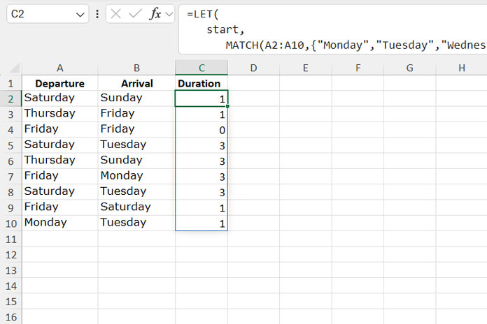
To calculate the days between the weekday names in A2:A10 (Departure) and B2:B10 (Arrival), enter the following formula in cell C2 after clearing C2:C10:
Excel:
=LET(
   start,
      MATCH(A2:A10,{"Monday", "Tuesday", "Wednesday", "Thursday", "Friday", "Saturday", "Sunday"}, 0),
   end,
      MATCH(B2:B10,{"Monday", "Tuesday", "Wednesday", "Thursday", "Friday", "Saturday", "Sunday"}, 0),
   IF(end>=start, end-start, 7-start+end)
)
Google Sheets:
Yes, this formula works in Google Sheets, but you need to use the ARRAYFORMULA function. Enter it as follows:
=ArrayFormula(LET(
   start,
      MATCH(A2:A10,{"Monday", "Tuesday", "Wednesday", "Thursday", "Friday", "Saturday", "Sunday"}, 0),
   end,
      MATCH(B2:B10,{"Monday", "Tuesday", "Wednesday", "Thursday", "Friday", "Saturday", "Sunday"}, 0),
   IF(end>=start, end-start, 7-start+end)
))
The formulas may return #N/A errors if any of the values are empty. This can be an issue when using larger ranges, such as A2:A1000 and B2:B1000, where only a few rows contain values.
To handle this, replace:
IF(end>=start,end-start,7-start+end)with:
IFNA(IF(end>=start,end-start,7-start+end),"")in both Excel and Google Sheets.