 in Google Sheets")

")

")


")


")


This tutorial is for users who want to apply XLOOKUP inside a structured table in Google Sheets (created via Insert > Table or Convert range to table). You’ll learn how to use both single and multiple conditions with structured references across two tables:
- A main (primary) table, where the formula is written.
- A lookup (reference) table, where the data is retrieved from.
Using structured references can make formulas cleaner and easier to manage—especially inside tables.
What Is “XLOOKUP Inside a Structured Table Row”?
It means writing an XLOOKUP formula that refers to structured column names within a table row, instead of traditional range references like A2:A10. This approach:
- Auto-expands to new rows (like Excel tables).
- Keeps formulas dynamic and readable.
- Supports both simple and multi-condition lookups.
Single Condition XLOOKUP in a Structured Table (Google Sheets Example)
Goal: Return the employee’s role from the lookup table based on the employee ID in the main table using structured references.
Table Structure:
Lookup Table (Table1):
| Employee ID | Role |
|---|---|
| EMP001 | Sales Associate |
| EMP002 | HR Manager |
| EMP003 | Software Engineer |
| EMP004 | Data Analyst |
| EMP005 | Marketing Lead |
Main Table (Table2):
| Employee ID | Role |
|---|---|
| EMP001 |
Formula in Table2[Role]:
=XLOOKUP(SINGLE(Table2[Employee ID]), Table1[Employee ID], Table1[Role])- The
SINGLE()function ensures only one value is passed toXLOOKUP. - The result auto-fills as new rows are added next to the last row.
Note: If you use the + (plus) button to insert a new row, the formula won’t auto-copy. Instead, type directly next to the last value.
ARRAYFORMULA with XLOOKUP in a Structured Table
If you prefer one formula that covers the entire column:
=ARRAYFORMULA(XLOOKUP(Table2[Employee ID], Table1[Employee ID], Table1[Role]))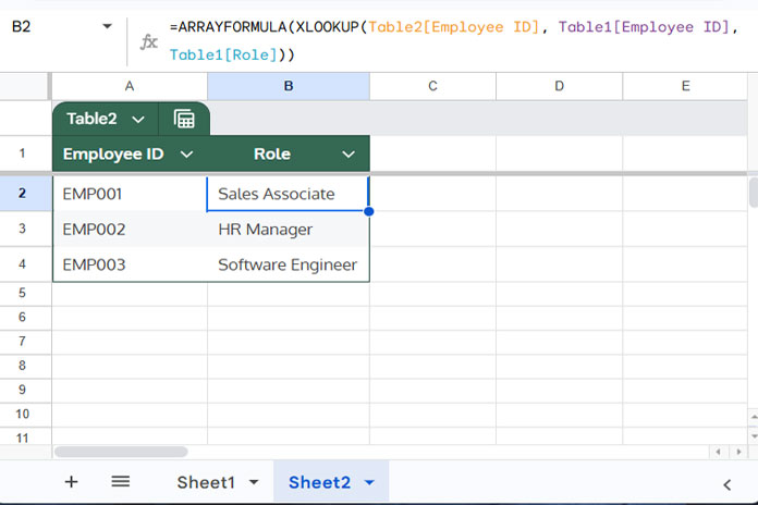
Multi-Condition XLOOKUP in Google Sheets Using Structured References
Goal: Return the product price by matching item, size, and color across two structured tables using multiple-condition XLOOKUP.
Table Structure:
Lookup Table (Table1):
| Employee ID | Role |
|---|---|
| EMP001 | Sales Associate |
| EMP002 | HR Manager |
| EMP003 | Software Engineer |
| EMP004 | Data Analyst |
| EMP005 | Marketing Lead |
Main Table (Table2):
| Item | Size | Color | Price |
|---|---|---|---|
| T-shirt | M | Red |
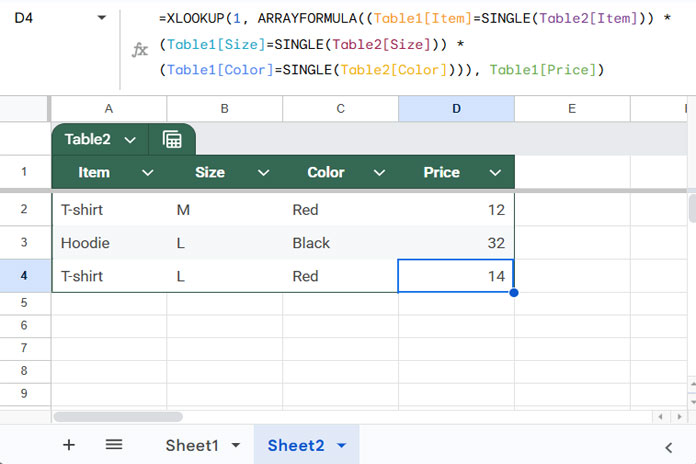
Formula (for one row):
=XLOOKUP(1, ARRAYFORMULA((Table1[Item]=SINGLE(Table2[Item])) * (Table1[Size]=SINGLE(Table2[Size])) * (Table1[Color]=SINGLE(Table2[Color]))), Table1[Price])Explanation:
- Each condition returns TRUE (1) or FALSE (0).
- All TRUEs multiply to 1.
XLOOKUPsearches for1and returns the corresponding price.
Array Formula for Multi-Condition XLOOKUP in Google Sheets
To make it work across all rows in Table2:
=MAP(Table2[Item], Table2[Size], Table2[Color], LAMBDA(x, y, z, XLOOKUP(1, ARRAYFORMULA((Table1[Item]=SINGLE(x)) * (Table1[Size]=SINGLE(y)) * (Table1[Color]=SINGLE(z))), Table1[Price])))MAPiterates over each row.LAMBDAcreates dynamic row-based XLOOKUP logic.
Alternative Method for Multi-Criteria XLOOKUP (Using Text Join)
You could combine the lookup conditions using & and search a concatenated column:
=ARRAYFORMULA(XLOOKUP(Table2[Item]&Table2[Size]&Table2[Color], Table1[Item]&Table1[Size]&Table1[Color], Table1[Price]))Summary
In this tutorial, you learned how to use XLOOKUP inside a structured table in Google Sheets, both for single-condition and multiple-condition lookups. With structured references and dynamic array formulas like ARRAYFORMULA and MAP, your lookups stay clean, scalable, and easy to manage.