This guide explains how to use the WRAPROWS function in Google Sheets, which is part of the suite of new functions introduced in early 2023, mostly under the “Array” category.

Purpose of the WRAPROWS Function

The WRAPROWS function wraps a given range of values (row or column) into multiple rows. Before WRAPROWS, there wasn’t a direct way to achieve this, and users had to rely on workarounds.

The difference between WRAPROWS and its counterpart, WRAPCOLS, is that WRAPROWS arranges values into rows, while WRAPCOLS arranges them into columns.

Syntax and Arguments

Syntax:

WRAPROWS(range, wrap_count, [pad_with])

• range: The range of values to wrap (a single row or column).
• wrap_count: The number of cells for each row in the output.
• pad_with (optional): Specifies what to fill any extra cells with. If omitted, the default is #N/A.

Examples

Let’s explore some practical examples.

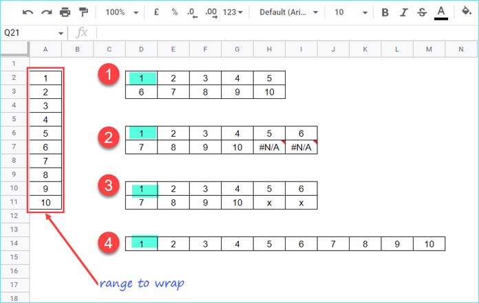
1. Wrap a Range with 5 Cells Per Row:
   =WRAPROWS(A2:A11, 5)
   This will arrange the values from A2:A11 into rows with 5 values per row.
2. Wrap a Range with 6 Cells Per Row:
   =WRAPROWS(A2:A11, 6)
   Since there are only 10 values, two #N/A errors appear in the second row.
3. Wrap with 6 Cells Per Row and Handle Extra Cells:
   =WRAPROWS(A2:A11, 6, "x")
   Since the range has only 10 values, two extra cells will be filled with “x.”
4. Exact Match of Wrap Count and Range:
   =WRAPROWS(A2:A11, 10)
   Here, the range has 10 values and is wrapped with exactly 10 cells per row, so no padding is needed.

Real-Life Application of WRAPROWS Function: Unstacking Data

One powerful use case of WRAPROWS is unstacking data. Suppose you have categories in column A and corresponding values in column B. If each category has the same number of rows, WRAPROWS can help you restructure the data into a more readable format.

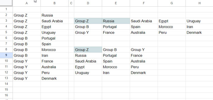
For instance:

In D3, use:

=UNIQUE(A2:A13)

In E3, use:

=WRAPROWS(B2:B13, 4)

This creates a table with unique categories and their corresponding values arranged horizontally.

To rearrange the output, you can combine functions like HSTACK and TRANSPOSE:

=TRANSPOSE(HSTACK(UNIQUE(A2:A13), WRAPROWS(B2:B13, 4)))

This formula transposes the combined output, making it easier to view.

Additional Tip: Expanding an Array with Empty Cells

If you’re an advanced Google Sheets user, you may need to add empty cells to array outputs, like shifting a dynamic calendar based on the day of the week. The WRAPROWS function can help with this.

For example, the formula below returns an array with 5 empty cells:

=IFNA(WRAPROWS(, 5))

You can combine this with an IF logical test to dynamically adjust the number of blank cells, offering great flexibility in various scenarios.

Handling Errors in the WRAPROWS Function

Common errors include:

• #N/A: Appears if you omit the pad_with argument when there aren’t enough elements to fill the final row. You can customize this by specifying a value for pad_with.
• #VALUE!: This error occurs if you mistakenly provide a 2D array to the WRAPROWS function, as it only accepts a single row or column as input.

This tutorial covers the essential use of the WRAPROWS function, providing practical examples and tips for handling errors and unstacking data.