


In Google Sheets Vlookup function, the range to consider for the search (the first column normally) can be a physical range or virtual range (an expression or other formula). The virtual range is useful when we want to Vlookup only in the last record in each group of data in Google Sheets.
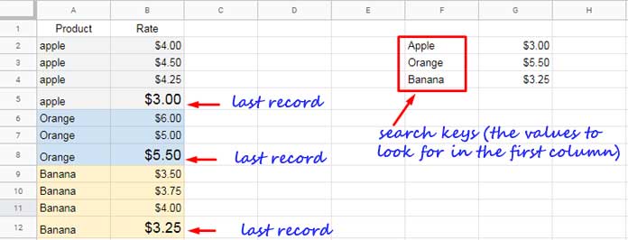
In the below example (screenshot), I have marked the last records in each group. I hope that will help you to understand what is the said last records in groups. I want to use the search keys in Vlookup to lookup in those records only.
Example to Vlookup Last Record in Each Group in Google Sheets (Screenshot):
Do you have an unsorted group in your table (range)? Don’t worry! The formula that I am going to provide in this tutorial will equally work in unsorted groups.
As you can see, I have my search keys in the array F2:F5. Yes! There are multiple search keys to lookup and I want only one Vlookup formula in cell G2 which expands.
I don’t want the formula to manually drag down. In other words, I want a Vlookup array formula that works in this specific scenario and can return an array output.
Formula Using One Search Key in Single Group
If I want to use only one search key, for example, “Apple”, I’ll use a Lookup function based formula instead of Vlookup. Here is that.
=ArrayFormula(lookup(1,1/SEARCH(F2,A2:A12),B2:B12))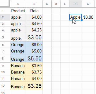
Similar: Lookup to Find the Last Occurrence of Multiple Criteria in Google Sheets (two or more criteria from the same row).
How to Vlookup Only in the Last Record in Each Group in Google Sheets
The Lookup formula in the just above example won’t work with multiple criteria (criteria from one column but from different groups). We can use the Vlookup function for that.
Then how to Vlookup only in the last record in each group using multiple search keys in Google Sheets?
I am trying to explain that here. Please read on and post if you have any queries at the end that in the comment section.
First of all, let me explain the logic involved. As I have mentioned, in Vlookup we can use a virtual ‘range‘ (expression).
Syntax:VLOOKUP(search_key, range, index, [is_sorted])As per my example, the physical range is A2:B. We can extract the last record from each group from this range and use that as a virtual range in Vlookup. That’s the key logic that I am using here.
Then how can we extract the last records from each group?
The SORTN function can remove the duplicate rows (Tie mode # 2). But it can thus only retain the first records.
Here we want to Vlookup (vertical lookup) in the last record in each group in Google Sheets.
Extracting First Records From Each Group
SORTN formula that retains first records:
=sortn(A2:B,9^9,2,1,0)
This formula retains the first record in each group. To get the last record, I have used the below workaround.
Extracting Last Records From Each Group to Use as Vlookup Range
The logic here is to move the last records to the top and then delete the duplicate records. How to do that?
That we can achieve by adding row numbers to the range A2:B as a new column and sort that column in descending order.
=sort({A2:B,if(len(A2:A),row(A2:A),"")},3,false)This moves the last records to the top. Then use it as the range in SORTN to retain the rows that we want.
=sortn(sort({A2:B,if(len(A2:A),row(A2:A),"")},3,false),9^9,2,1,false)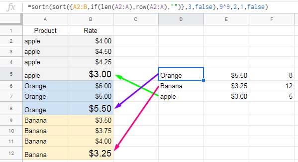
If you find this difficult to grasp, nothing to worry about. See the detailed tutorial here – How to Find the Last Row in Each Group in Google Sheets.
Vlookup Only in the Last Records in Google Sheets (Formula and Explanation)
We have now the virtual range, which is the SORTN formula above, to use in Vlookup to lookup the last record in each group in Google Sheets.
Here is the Vlookup formula that uses that virtual range (expression).
=ArrayFormula(vlookup(F2:F4,sortn(sort({A2:B,if(len(A2:A),row(A2:A),"")},3,false),9^9,2,1,false),2,0))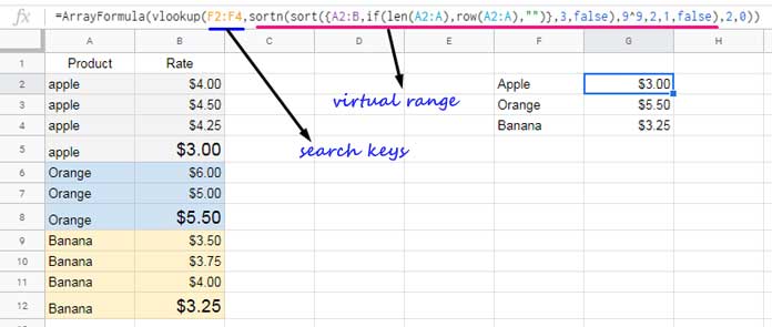
For the formula explanation, see the illustration above.
That’s all about how to use Vlookup only in the last records in each group in Google Sheets.
Thanks for the stay. Enjoy!