


I know I should start this tutorial by explaining the term Vlookup Identical String Match in the title. So we will start from that.
It’s related to the Vlookup search key and the search column (first column in the range)
E.g., usually, the search key “Train” will match the strings “train,” “TRAIN,” “Train,” etc.
But we want to match only the string “Train” as they share identical characters and cases.
We can use the EXACT function in Google Sheets for such comparison.
We have already learned to use the said function for Vlookup identical string match, and here is that tutorial – Case Sensitive Vlookup in Google Sheets [Solved].
But it is a non-array solution and won’t support multiple search keys in one formula.
This post contains the array version.
In short, this post is about the case-sensitive Vlookup array formula. We can also say multiple criteria Vlookup EXACT match.
Here we go!
Sample Data, Criteria, and Vlookup Identical String Match
Sample Data for Multiple Criteria Vlookup EXACT Match:
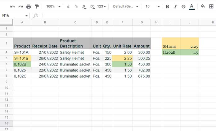
The lookup range and output ranges are A4:A (Product) and F4:F (Unit Rate), respectively.
The lookup criteria/search keys are in I3:I4.
The goal is to search the criteria (I3:I4) in the table (A4:G) and return their unit rates.
Let’s code an array formula to Vlookup identical string match in Google Sheets.
Vlookup Identical String Match Array Formula
I have used the following Vlookup Identical String Match Array Formula in cell J3.
=ArrayFormula(vlookup(I3:I4&TRUE,{A4:A®exmatch(A4:A,"^"&textjoin("$|^",true,I3:I4)&"$"),B4:G},6,0))How does this Vlookup formula perform EXACT match multiple criteria in Google Sheets?
Note:- Here exact means case-sensitive or match by character and case.
Here is the walk-through.
Formula Explanation
To learn the Vlookup identical string match array Formula, peel it to take the inner part and enter it in a blank column. Here it is.
Step 1:
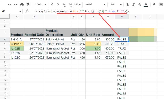
Part_1: regexmatch(A4:A,"^"&textjoin("$|^",true,I3:I4)&"$")
Enter the above part in cell H4 as below.
=ArrayFormula(regexmatch(A4:A,"^"&textjoin("$|^",true,I3:I4)&"$"))It will match the two search keys in I3:I4 in A4:A and return TRUE for the match and FALSE for the mismatch.
It’s case sensitive and exact (not partial) match; collectively known as an identical string match.
E.g.:
Case Sensitive – The search key “Train” will match with “Train.” Not with “TRAIN” or “train.”
Exact Match – The search key “Train” will match with “Train,” not with “Bullet Train.”
Step 2:
To understand the rest of the formula parts, please follow this Vlookup syntax in use here.
Syntax:- =Array_Formula(VLOOKUP(search_key, range, index, [is_sorted]))
Here are the actual parameters that we may use in a case-insensitive formula.
search_key – I3:I4
range – A4:G
index – 6 (unit rate column)
is_sorted – 0
We should modify them as below for Vlookup multiple criteria exact match aka identical string match and that is what I have done.
search_key – I3:I4&TRUE – it’s because, next, we will add the part_1 output with the search column (the first column in the range).
range – {A4:A&H4:H,B4:G}– replace H4:H with the corresponding formula (part_1).
index – 6 (unit rate column)
is_sorted – 0
That’s all. Thanks for the stay. Enjoy!
Resources
- How to Do a Case Sensitive Sumproduct in Google Sheets.
- How to Perform a Case Sensitive COUNTIF in Google Sheets.
- Case Sensitive Reverse Vlookup Using Index Match in Google Sheets.
- How to Do a Case Sensitive SUMIF in Google Sheets.
- How to Do a Case Sensitive DSUM in Google Sheets.