The Two-Way Filter in Google Sheets — What Does It Mean?
A two-way filter formula extracts rows and columns that meet given criteria or conditions. It can also be called a dynamic horizontal and vertical filter in Google Sheets.
To filter rows, you can use either the FILTER or QUERY function. But what about filtering columns, such as the header row?
While the FILTER function can filter columns, it cannot filter rows and columns simultaneously without using multiple filters. On the other hand, the QUERY function allows you to achieve both in a single formula when combined with the MATCH function.
In this tutorial, you will learn all about dynamic two-way vertical and horizontal filtering using QUERY and FILTER in Google Sheets.
Two-Way Filter in Google Sheets

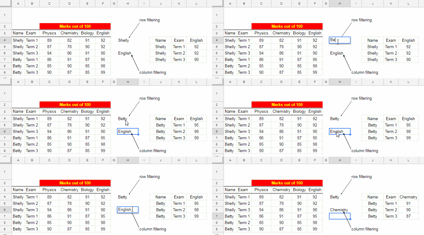
In the example of a two-way filter, we filter rows containing the name “Betty” in the range A3:A (row filter) and the subject “Chemistry” in the range A3:F3 (column filter).
Using QUERY
Here’s the formula in cell J4:
=QUERY(A3:F, "Select Col1, Col2, Col"&MATCH(H6, A3:F3, 0)&" where Col1='"&H4&"'")How to Use This Formula
A3:F: The data range.Select Col1, Col2: Two static columns containing Name (column A) and Exam (column B).MATCH(H6, A3:F3, 0): Finds the column number based on the criterion in cellH6.
You can omit the static columns by removing Col1, Col2, or keep only one of them. Here is an example:
=QUERY(A3:F, "Select Col1, Col"&MATCH(H6, A3:F3, 0)&" where Col1='"&H4&"'")These formulas filter rows and columns based on one condition each. The criterion for row filtering is in cell H4, and the criterion for column filtering is in cell H6.
In summary:
- Row filtering conditions are specified in the
WHEREclause. - Column selection is managed by manually specifying static columns and using the
MATCHfunction to dynamically include other columns.
Please note that the above formulas are case-sensitive. To make them case-insensitive, you should specify the row filter criterion in lowercase and include the LOWER function within the QUERY. In short, you should replace Col1='"&H4&"' with LOWER(Col1)='"&H4&"' and ensure that H4 contains the criterion in lowercase.
Using FILTER
Here’s how to create a two-way filter step by step:
- Filter Rows:
=FILTER(A3:F9, A3:A9=H4)This filters rows based on the name in column A matching the value in cell H4. However, it excludes the header row.
- Include the Header Row:
=VSTACK(A3:F3, FILTER(A3:F9, A3:A9=H4))This formula appends the header row at the top of the filtered rows using VSTACK, allowing you to filter columns based on the header row.
- Filter Columns:
=FILTER(VSTACK(A3:F3, FILTER(A3:F9, A3:A9=H4)), A3:F3=H6)This filters the columns that match the criterion in cell H6. This completes the two-way filtering.
- Include Static Columns:
To include specific static columns, use the following formula:
=FILTER(VSTACK(A3:F3, FILTER(A3:F9, A3:A9=H4)), (A3:F3=H6)+(A3:F3="Name")+(A3:F3="Exam"))This filters the required columns and ensures static columns (“Name” and “Exam”) are included.
Two-Way Filter in Google Sheets – Two Conditions in Row Filtering
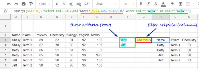
For this example, let’s filter rows based on two conditions and columns based on one condition. The data range is A2:G with headers in row 2.
QUERY Formula:
=QUERY(A2:G, "Select Col1, Col2, Col" & MATCH(J3, A2:G2, 0) & " where Col1='" & I3 & "' or Col1='" & I4 & "'")
Explanation:
Col1='" & I3 & "' or Col1='" & I4 & "'– Applies two conditions for row filtering using theORoperator.
FILTER Formula:
=FILTER(VSTACK(A2:G2, FILTER(A2:G, (A2:A=I3) + (A2:A=I4))), (A2:G2=J3) + (A2:G2="Name") + (A2:G2="Exam"))Breakdown:
FILTER(A2:G, (A2:A=I3) + (A2:A=I4))– Filters rows based on multiple conditions.VSTACK(A2:G2, ...)– Adds the header row to the result.FILTER(..., (A2:G2=J3) + (A2:G2="Name") + (A2:G2="Exam"))– Filters columns with static column inclusion.
Two-Way Filter in Google Sheets – Two or More Conditions in Column Filtering
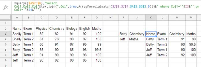
To filter two or more columns dynamically, you can use the following approach.
QUERY Approach
=QUERY(A2:G, "Select Col1, Col2, Col" & TEXTJOIN(",Col", TRUE, ARRAYFORMULA(MATCH(J3:J4, A2:G2, 0))) & " where Col1='" & I3 & "' or Col1='" & I4 & "'")
Explanation:
TEXTJOIN(",Col", TRUE, ARRAYFORMULA(MATCH(J3:J4, A2:G2, 0)))– Dynamically joins column references matching criteria in cellsJ3andJ4.- To add more columns, extend the range in
MATCH, e.g.,J3:J5.

FILTER Approach
=FILTER(VSTACK(A2:G2, FILTER(A2:G, (A2:A=I3) + (A2:A=I4))), (A2:G2=J3) + (A2:G2=J4) + (A2:G2="Name") + (A2:G2="Exam"))To include more columns, extend the conditions in the outer FILTER.
Conclusion
By now, you should have a solid understanding of how to implement a two-way filter in Google Sheets using both QUERY and FILTER functions. Whether filtering vertically, horizontally, or both, these methods offer flexibility and efficiency for dynamic data management.
Thanks for reading! Enjoy exploring the power of two-way filtering in Google Sheets!


