It’s easy to check whether test results fall within their limits in Google Sheets. You can use either the ISBETWEEN function or comparison operators. This tutorial will walk you through both approaches.

In such logical tests, typically three arrays are involved:

1. Actual results – the values to test.
2. Lower limit – start of the acceptable range.
3. Upper limit – end of the acceptable range.

For example, in a medical lab report, the Result column corresponds to the test results, while Range From and Range To columns represent the normal limits.

Similarly, in a job schedule, you might want to test whether actual start dates fall within scheduled start and end dates.

Example Dataset

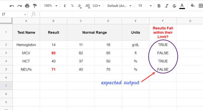
Here, we want to check if each Result falls between its corresponding Range From and Range To.

Solution 1: Using ISBETWEEN

Place this formula in cell F2:

=ISBETWEEN(B2:B5, C2:C5, D2:D5)

• B2:B5 → values to compare.
• C2:C5 → lower limits.
• D2:D5 → upper limits.

This will return TRUE for values within range and FALSE otherwise.

To handle dynamic ranges with possible blank rows, use:

=ARRAYFORMULA(IF(LEN(B2:B), ISBETWEEN(B2:B, C2:C, D2:D), ))

This ensures the formula only evaluates rows with actual data.

Solution 2: Using Comparison Operators

You can achieve the same result using comparison operators:

=ARRAYFORMULA(IF((B2:B5>=C2:C5)*(B2:B5<=D2:D5), TRUE, FALSE))

Or, for dynamic ranges:

=ARRAYFORMULA(IF(LEN(B2:B), IF((B2:B>=C2:C)*(B2:B<=D2:D), TRUE, FALSE), ))

Both formulas return TRUE if the result falls within the limits, FALSE otherwise.

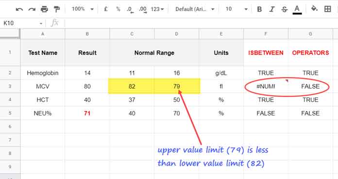
Why ISBETWEEN is Recommended:

• Simpler to read and learn.
• Automatically returns #NUM! if the lower limit is greater than the upper limit, which helps catch data errors.

Highlight Out-of-Range Test Results

To highlight values outside their limits using conditional formatting:

1. Select cell B2.
2. Go to Format → Conditional formatting.
3. Set Apply to range: B2:B1000.
4. Under Format rules, choose Custom formula is.
5. Enter:

=ISBETWEEN($B2, $C2, $D2)=FALSE

6. Set the formatting style (e.g., red text, bold).
7. Click Done.

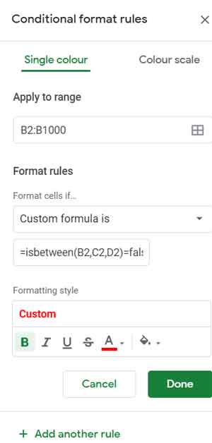
This highlights all results that do not fall within their range.

Key Takeaways

• Use ISBETWEEN to easily test if values fall within a range.
• Comparison operators provide an alternative, but formulas are more complex.
• ISBETWEEN works with numbers, dates, or text, and handles multiple arrays.
• Conditional formatting can flag out-of-range values visually.

Resources

• Visually Track Where Your Data Falls Within Limits (Google Sheets)
• ISBETWEEN Function in Conditional Formatting in Google Sheets
• How to Use ISBETWEEN with FILTER Formula in Google Sheets
• COUNTIFS with ISBETWEEN in Google Sheets