


")


")

")
")
 in Excel & Google Sheets")


In Google Sheets, we can summarize data (like sum, average, min, max, count) using the QUERY function, but how do we also keep the last record along with the summary? This can be achieved using a combination of the QUERY and SORTN functions, with some helper functions to facilitate the task.
Summarizing data while retaining the last record provides both a summary of the overall data and details from the most recent observation. However, coding a formula for this can vary depending on the data structure and requirements.
In this tutorial, I’ll walk you through two solutions to address different scenarios, including grouping by a single column or multiple columns. Let’s dive in and learn how to handle these scenarios with ease.
Sample Data
Here is some sample data prepared specifically for this tutorial. It’s a typical sales dataset containing the following columns:
- Date: Date of the sale
- Name: Salesperson’s name
- Item: Item sold
- Sales: Quantity sold
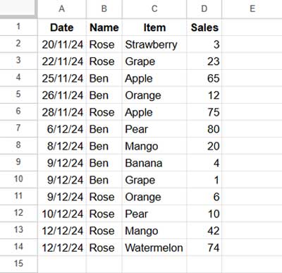
Ensure your dataset has no empty rows between records.
Do We Need to Sort the Data?
We assume your data is entered in the sequence of events, with earlier records at the top and the latest records at the bottom. In this case, sorting is not required.
If the data order is reversed, you may need to flip it. To do this:
- Manually enter sequential numbers in a new column.
- Enter 1 in E2 and 2 in E3, then select both cells and drag the fill handle down to complete the sequence.
- Select your data range (e.g., A2:E14).
- Click Data > Sort Range > Advanced range sorting options.
- Sort by column E in Z → A order.
- You can then remove the sequential numbers in column E.
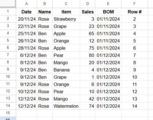
Adding Two Helper Columns: BOM and Row Numbers
Adding helper columns simplifies the formulas. BOM (Beginning of the Month) converts sales dates to the first day of the month for monthly grouping.
- BOM Helper Column (Column E): Enter the following formula in E2:
=ArrayFormula(TO_DATE(IFERROR(EOMONTH(DATEVALUE(A2:A), -1) + 1))) - Row Numbers Helper Column (Column F): Enter the following formula in F2:
=ArrayFormula(IF(A2:A="", , ROW(A2:A)))
Although we could embed these calculations directly into the final formulas, using helper columns makes the formulas easier to read and understand.
Level 1: Summarize Data by Name and Keep the Last Record
This is the simplest case, with grouping by a single column (Name).
Step 1: Create the Summary
Use the QUERY function to group the data by the Name column and sum the Sales column:
=QUERY(A2:D, "SELECT B, SUM(D) WHERE A IS NOT NULL GROUP BY B LABEL SUM(D)''", 0)This groups by column B (Name) and aggregates the sales (column D). You can replace SUM with other aggregation functions like COUNT, MIN, MAX, or AVG as needed.
The formula would return the following result:
| Ben | 182 |
| Rose | 233 |
Step 2: Retain the Last Record
Use the following formula to retrieve the last record for each group:
=SORTN(SORT(FILTER(A2:F, A2:A<>""), 2, 1, 6, 0), 9^9, 2, 2, 1)The output will match the number of rows returned by the query formula in Step 1. Here’s the result:
| 9/12/24 | Ben | Grape | 1 | 01/12/2024 | 10 |
| 12/12/24 | Rose | Watermelon | 74 | 01/12/2024 | 14 |
Explanation:
- FILTER removes empty rows from the range.
- SORT sorts by the Name column (column 2) in ascending order and by the Row Numbers column (column 6) in descending order. This ensures the last record of each group appears at the top of the group.
- SORTN removes duplicates (based on Name) and retains the last record of each group.
Syntax of SORTN:
SORTN(range, [n], [display_ties_mode], [sort_column], [is_ascending], [sort_column2, …], [is_ascending2, …])Where:
range: The output of the SORT formula.n: The number of rows to return; here,9^9is used as an arbitrarily large number to ensure all groups are included.display_ties_mode: Set to2to remove duplicates.sort_column: Refers to column 2, which is the grouping column used in the QUERY formula.is_ascending: Set to1to sort thesort_columnin ascending order.
This formula effectively retrieves the last record for each group, maintaining alignment with the grouped summary from Step 1.
Step 3: Combine Results
Combine the summary (Step 1) and last record results (Step 2) using HSTACK:
=HSTACK(
   QUERY(A2:D, "SELECT B, SUM(D) WHERE A IS NOT NULL GROUP BY B LABEL SUM(D)''", 0),
   SORTN(SORT(FILTER(A2:F, A2:A<>""), 2, 1, 6, 0), 9^9, 2, 2, 1)
)
This formula effectively summarizes the data and retains the last rows for each group. However, it includes some unwanted columns. In the next step, we will refine the result by selecting only the columns we need.
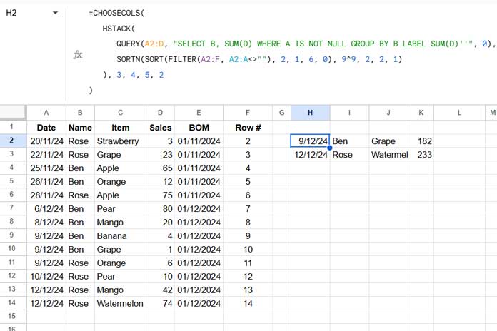
Step 4: Choose Columns
Select the columns you want to display using CHOOSECOLS:
=CHOOSECOLS(
   HSTACK(
      QUERY(A2:D, "SELECT B, SUM(D) WHERE A IS NOT NULL GROUP BY B LABEL SUM(D)''", 0),
      SORTN(SORT(FILTER(A2:F, A2:A<>""), 2, 1, 6, 0), 9^9, 2, 2, 1)
   ), 3, 4, 5, 2
)
In this case, columns 3, 4, 5, and 2 represent the last sales date, salesperson’s name, sold item, and total sales quantity, respectively.
Level 2: Summarize Data by Name and Month and Keep the Last Record
In the previous example, we summarized the data by the Name column and retained the last record, which involved only a single grouping column. Here, we’ll look at an example with two-column grouping and retain the most recent record.
For grouping by multiple columns (e.g., Name and Month), the approach is similar, with minor adjustments.
Step 1: Create the Summary
Group the data by Name and BOM (helper column E):
=QUERY(A2:E, "SELECT B, E, SUM(D) WHERE A IS NOT NULL GROUP BY B, E LABEL SUM(D)''", 0)Step 2: Retain the Last Record
Adjust the SORTN formula to include the BOM column:
=SORTN(SORT(FILTER(A2:F, A2:A<>""), 2, 1, 6, 0), 9^9, 2, 2, 1, 5, 1)Combine Results and Choose Columns
Follow steps 3 and 4 as in Level 1 (example 1), updating the columns in the CHOOSECOLS part as needed.
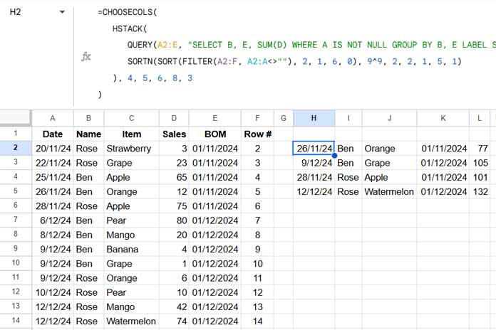
Here’s the combined formula:
=CHOOSECOLS(
   HSTACK(
      QUERY(A2:E, "SELECT B, E, SUM(D) WHERE A IS NOT NULL GROUP BY B, E LABEL SUM(D)''", 0),
      SORTN(SORT(FILTER(A2:F, A2:A<>""), 2, 1, 6, 0), 9^9, 2, 2, 1, 5, 1)
   ), 4, 5, 8, 3
)
This formula returns the most recent sales date, salesperson’s name, last sold item, month, and total sales quantity.
Note: When summarizing data by Name and Month (BOM) to keep the last record as shown above, the Month column contains the beginning-of-the-month dates. You can format this column to display as “mmm-yy” by selecting it and navigating to Format > Number > Custom Number Format.
Wrap-Up
Summarizing data and retaining the last record in Google Sheets is straightforward with the right combination of functions.
- Use QUERY for grouping and summarizing data.
- Use SORTN to retain the last record of each group.
- Combine results using HSTACK and select desired columns with CHOOSECOLS.
By following these steps, you can handle various grouping scenarios and maintain a clear sequence in your data.