When it comes to summing, multiplying, subtracting, and dividing numbers in Google Sheets, you have multiple options. You can use either built-in functions or equivalent arithmetic operators. This post explains both methods, with a focus on functions.

Total a Column, Row, or Range

Use the SUM function to total a row, column, range, or a series of hardcoded numbers.

Syntax of the SUM Function in Google Sheets

SUM(value1, [value2, ...])

• value1: The first number to add.
• value2, …: Additional numbers to add to value1.

The argument value2, ... is optional, and you can specify column, row, or range references in value1 and value2, .... The size of the row, column, or range can vary. Also, note that the function ignores any text within the specified range.

Examples of Using the SUM Function in Google Sheets

=SUM(B2:B5)

Returns the total of the numbers in the range B2:B5. This is a closed range.

If you want to total an entire column starting from B5 downwards, use:

=SUM(B5:B)

Similarly, to sum values in a row range:

=SUM(A2:E2)

Returns the total of the numbers in A2:E2.

The following formula returns the total of all numbers in row #2.

=SUM(2:2)

Additional Examples

=SUM(10, 20, 30) // returns 60
=SUM(B2:C10) // returns the total of values in columns B and C

Add Two Numbers

To add two numbers, use the ADD function or the equivalent + arithmetic operator.

Syntax of the ADD Function in Google Sheets

ADD(value1, value2)

• value1 – The first number.
• value2 – The second number to add.

Examples of the ADD Function and the + Operator

=ADD(5, 10) // returns 15

Equivalent: =5+10

=ADD(A1, B1)

Equivalent: =A1+B1

If one or both values are text, the formula returns a #VALUE! error. If more than two arguments are provided, it returns a #N/A error.

For row-wise addition:

=ArrayFormula(ADD(B2:B10, C2:C10))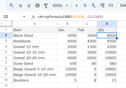

The formula sums the total sales in January and February from B2:B10 and C2:C10, placing the results in D2:D10.

Equivalent formula:

=ArrayFormula(B2:B10+C2:C10)

Subtract Two Numbers

Use the MINUS function or the - arithmetic operator.

Syntax of the MINUS Function in Google Sheets

MINUS(value1, value2)

• value1 – The first number.
• value2 – The second number subtracted from value1.

Examples of the MINUS Function and the – Operator

=MINUS(10, 5) // returns 5

Equivalent: =10-5

=MINUS(A1, B1)

Equivalent: =A1-B1

The same error rules as the ADD function apply here (#VALUE! for text, #N/A for more than two arguments).

For row-wise subtraction:

=ArrayFormula(MINUS(B2:B10, C2:C10))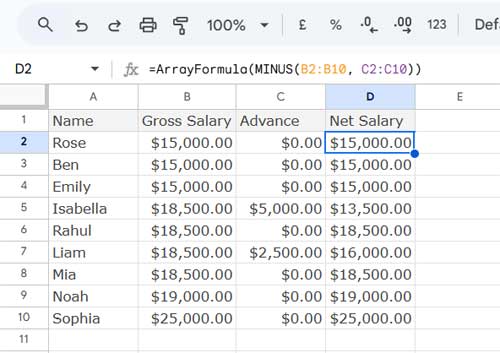

The formula returns the net salary by subtracting the advance in C2:C10 from the gross salary in B2:B10.

Equivalent formula:

=ArrayFormula(B2:B10-C2:C10)

Multiply Two Numbers

Use the MULTIPLY function or the * operator.

Syntax of the MULTIPLY Function in Google Sheets

MULTIPLY(factor1, factor2)

• factor1 – The first value.
• factor2 – The second value to multiply.

Examples of the MULTIPLY Function and the * Operator

=MULTIPLY(10, 5) // returns 50

Equivalent: =10*5

=MULTIPLY(A1, B1) // multiplies values in A1 and B1

Equivalent: =A1*B1

Errors:

• #VALUE! if one or both values are text.
• #N/A if more than two arguments are provided.

For row-wise multiplication:

=ArrayFormula(MULTIPLY(B2:B10, C2:C10))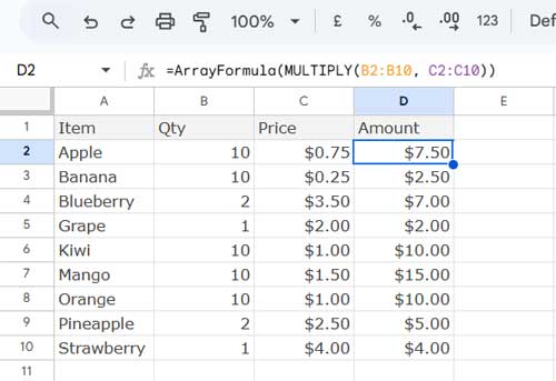

In this example, the formula calculates the amount for each item in A2:A10 by multiplying the quantity in B2:B10 with the price in C2:C10.

Equivalent formula:

=ArrayFormula(B2:B10*C2:C10)

Divide Two Numbers

Use the DIVIDE function or the / operator.

Syntax of the DIVIDE Function in Google Sheets

DIVIDE(dividend, divisor)

• dividend – The number to be divided.
• divisor – The number to divide by.

Examples of the DIVIDE Function and the / Operator

=DIVIDE(100, 50) // returns 2

Equivalent: =100/50

=DIVIDE(A1, B1) // divides A1 by B1

Equivalent: =A1/B1

Errors:

• #VALUE! if one or both numbers are text.
• #DIV/0! if the divisor is 0.
• #N/A if more than two arguments are provided.

For row-wise division:

=ArrayFormula(DIVIDE(B2:B10, C2:C10))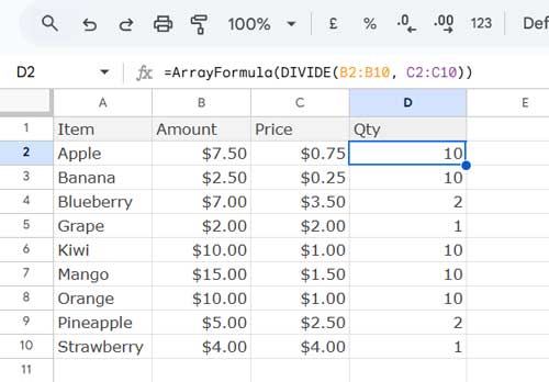

The formula returns the quantities by dividing the amount in B2:B10 by the price in C2:C10.

Equivalent formula:

=ArrayFormula(B2:B10/C2:C10)

Wrap-Up

We’ve covered how to sum, multiply, subtract, and divide in Google Sheets using both functions and arithmetic operators.

The ADD, MINUS, MULTIPLY, and DIVIDE functions take two arguments and return a single value. However, you can specify two one-dimensional ranges to get row-wise results.

When using arithmetic operators, you can specify more than two values or one-dimensional ranges. For example:

=ArrayFormula(B2:B10*C2:C10*D2:D10) or =B2*C2*D2

The SUM function allows multiple arguments and returns a single value.

These formulas make it easy to handle calculations efficiently in Google Sheets.

Resources

• How to Use Arithmetic Operators in QUERY in Google Sheets
• How to Use UNIQUE and SUM Together in Google Sheets
• Sum Cells With Numbers and Text in a Column in Google Sheets
• Extract All Numbers from Text and Sum Them in Google Sheets
• Subtract a Duration from Duration in Google Sheets
• How to Subtract the Previous Value from the Current Value in Google Sheets