Summing the Largest N Values by Group in Google Sheets

You can easily sum the largest N values by group in Google Sheets using a combination of SORT, COUNTIFS and QUERY. This technique is useful in various fields such as education, sales, sports, and more.

For example, you can use this method to:

Consider only the top N subject scores for student admissions.
Calculate the best N months’ total sales for a salesperson.
Sum the fastest N race times for qualification rankings.
And many other use cases!

Generic Formula

=LET(
   category, A2:A, score, B2:B, n, 3, 
   rangeS, SORT(HSTACK(category, score), 1, TRUE, 2, FALSE), 
   rcS, ARRAYFORMULA(COUNTIFS(SORT(category, 1, TRUE, score, FALSE), SORT(category, 1, TRUE, score, FALSE), ROW(category), "<="&ROW(category))), 
   ftr, FILTER(rangeS, rcS<=n), 
   QUERY(ftr,"SELECT Col1, SUM(Col2) WHERE Col1 IS NOT NULL GROUP BY Col1 LABEL SUM(Col2)''")
)

How to Use This Formula?

Replace A2:A with the category column reference (e.g., Student Names).
Replace B2:B with the score column reference (e.g., Marks or Sales).
Replace 3 with your desired value of N (e.g., sum the largest 3 values per group).

This formula will instantly sum the largest N values by category, generating a summary in one step!

Example: Summing the Largest N Values by Group in Google Sheets

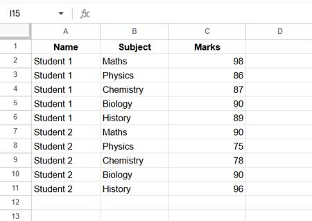
Consider the following dataset, which contains student names, subjects, and marks:

Sample dataset for summing the largest N values by group

Goal:

We want to sum the highest 3 subject scores for each student.

Formula for This Example:

=LET(
   category, A2:A, score, C2:C, n, 3, 
   rangeS, SORT(HSTACK(category, score), 1, TRUE, 2, FALSE), 
   rcS, ARRAYFORMULA(COUNTIFS(SORT(category, 1, TRUE, score, FALSE), SORT(category, 1, TRUE, score, FALSE), ROW(category), "<="&ROW(category))), 
   ftr, FILTER(rangeS, rcS<=n), 
   QUERY(ftr,"SELECT Col1, SUM(Col2) WHERE Col1 IS NOT NULL GROUP BY Col1 LABEL SUM(Col2)''")
)

Explanation:

A2:A represents the category (student names).
C2:C represents the score (marks).
3 means we are summing the top 3 scores for each student.

Output:

Student 1	277
Student 2	276

Formula Logic & Breakdown

1. Sorting the Data

SORT(HSTACK(category, score), 1, TRUE, 2, FALSE)

Sorts data by category (A-Z).
Sorts scores in descending order (so the highest scores appear first).

Name	Marks
Student 1	98
Student 1	90
Student 1	89
Student 1	87
Student 1	86
Student 2	96
Student 2	90
Student 2	90
Student 2	78
Student 2	75

2. Assigning a Running Count

ARRAYFORMULA(COUNTIFS(SORT(category, 1, TRUE, score, FALSE), 
SORT(category, 1, TRUE, score, FALSE), ROW(category), "<="&ROW(category)))

Assigns a rank to each score within its category.
Ensures that only the top N values are selected for summation.

3. Filtering the Top N Scores

FILTER(rangeS, rcS<=n)

Keeps only the highest N values per group.

Name	Marks
Student 1	98
Student 1	90
Student 1	89
Student 2	96
Student 2	90
Student 2	90

4. Summing the Largest N Values by Group

QUERY(ftr, "SELECT Col1, SUM(Col2) WHERE Col1 IS NOT NULL GROUP BY Col1 LABEL SUM(Col2)''")

Groups data by category (student name).
Computes the sum of the highest N scores per category.

Why Use This Method?

This approach works seamlessly with both sorted and unsorted data, making it highly flexible.

It can handle any number of groups or categories, allowing you to sum the largest N values by category dynamically.

Best of all, it eliminates the need for manual filtering or sorting, saving time and effort while ensuring accuracy.

🔹 How to Find the Highest N Values in Each Group in Google Sheets
🔹 How to Filter Top 10 Items in a Google Sheets Pivot Table