


")


")

")
")
 in Excel & Google Sheets")


If you don’t need pattern matching and want a simple text replacement in Google Sheets, SUBSTITUTE is the function to look for. Otherwise, you should check out REGEXREPLACE.
The purpose of the SUBSTITUTE function is to replace existing text with new text in a string. Let’s see how to use this function in Google Sheets.
Syntax and Arguments of the SUBSTITUTE Function
Syntax:
SUBSTITUTE(text_to_search, search_for, replace_with, [occurrence_number])Arguments:
text_to_search: The text in which to search and replace.search_for: The string to search for.replace_with: The string that will replace the matching search string. Matching is case-sensitive.occurrence_number: The occurrence of the search string to be replaced. This is optional and if omitted, all occurrences will be substituted.
Examples
Let’s use the following sentence as text_to_search:
“We are looking for light green trousers, a black T-shirt, and dark green socks.”
Assume it’s in cell A1.
The following formula will replace all occurrences of “green” (search_for) with “blue” (replace_with):
=SUBSTITUTE(A1, "green", "blue")Output: “We are looking for light blue trousers, a black T-shirt, and dark blue socks.”
If you want to replace only the first occurrence of “green”, i.e., in “green trousers”, use the following formula:
=SUBSTITUTE(A1, "green", "blue", 1)Output: “We are looking for light blue trousers, a black T-shirt, and dark green socks.”
Using the SUBSTITUTE function is that simple in Google Sheets.
SUBSTITUTE Function: Advanced Techniques and Best Practices
Here are some tips and tricks that will help you when using the SUBSTITUTE function extensively in Google Sheets:
- When you want to search and remove a string, specify the replacement with an empty string (
""). - Sometimes you might want to include a white space prefix before the search string. For example, if you want to replace “apple” but not “apple” in “pineapple”, you may consider adding a space before “apple” in the search string, like
" apple". - You can repeat a string ‘n’ times using the SUBSTITUTE function in Google Sheets. Specify
""(empty string) in bothsearch_forandreplace_withand use a SEQUENCE formula inoccurrence_number.
Example:
=ArrayFormula(SUBSTITUTE(A1, "", "", SEQUENCE(1, 5)))This formula will repeat the text in cell A1 five times.
Streamlining OR Logic: Efficient Search Key Substitution
XLOOKUP is one of the popular options for lookup in Google Sheets.
Assume you have fruit names in column A and their corresponding expected arrival dates in column B. The data is sorted in ascending order based on the arrival dates.
To find the first arrival date of “Melon”, you can use the following formula:
=XLOOKUP("Melon", A:A, B:B)And this one will return the first arrival date of “Blueberry”:
=XLOOKUP("Blueberry", A:A, B:B)When you look through both results, you can find which one you receive first. If you want to do this in a single XLOOKUP, you can replace “Melon” in the range A:A with “Blueberry” and use that as the lookup range:
=ArrayFormula(XLOOKUP("Blueberry", SUBSTITUTE(A:A, "Melon", "Blueberry"), B:B))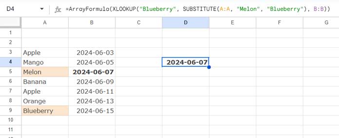
Here we apply the SUBSTITUTE function in a column. So we must use the ARRAYFORMULA function as above.
Resources
Here are some relevant Google Sheets resources.
- How to Count Comma Separated Words in a Cell in Google Sheets
- Substitute Nth Match of a Delimiter from the End of a String in Google Sheets
- Replace Multiple Comma Separated Values in Google Sheets
- Extract, Replace, Match Nth Occurrence of a String or Number in Google Sheets
- How to Replace Every Nth Delimiter in Google Sheets
- Remove or Replace Last Character from a String in Google Sheets
Hi,
How do replace a value and have the replacement appear in the same box that the value initially was? I notice that Substitute always shows up in its own box. For example, I have 0 in box A1 and want to replace 0 with 1 so that box A1 becomes 1. I want to do this on a very large scale and need to do it with formulas. Do you have any suggestions?
Thanks.
Hi, Les,
You won’t be able to do that using a formula. You can use the Edit > Find and Replace command (Ctrl+H) or an Apps Script. I don’t have the script for the same.
Hi There:
I have a cell that has two texts that I need to eliminate to obtain a number; for instance, US$250.00$, I want to substitute “US$” and “$” all at once.
I have been able to do it separately using the following formulas
=SUBSTITUTE(H4,"US$","")and=SUBSTITUTE(I4,"$","").I would like to know if I can combine both formulas into one to make the work easier.
Thanks
Hi, Cruz A Villasana,
You can either nest the two Substitute formulas or use a Regexreplace formula instead.
Using Substitute:
=substitute(SUBSTITUTE(H4,"US$",""),"$","")*1Using Regexreplace:
=REGEXREPLACE(H4, "[^\d\.-]+", "")*1